State Budget Gaps and State Budget Growth

For the past two fiscal cycles, states have grappled with unprecedentedly large budget gaps. By the simple arithmetic of fiscal policy, these gaps can be closed with budget cuts or revenue increases. An important question for the policy maker is: Which of these two courses of action is likely to spur further budget gaps in future years? In this paper, I examine this question by looking at state policies and institutions in the decades preceding the budget gaps. I find that state governments that spent a larger fraction of state income—and had done so for many decades—experienced smaller percentage budget gaps in FY2010. On the other hand, states whose per capita spending levels increased the most over the last two decades had larger percentage budget gaps in FY2010. Furthermore, states whose policies permit economic freedom and states with strict balanced budget requirements experienced smaller budget gaps. Taken together, these results suggest that spending restraint, economic freedom, and institutional rules that ensure a strict balanced budget requirement seem to be a more reliable path to fiscal balance than tax increases.¹

Section I. Introduction

Following the economic collapse of 2008, nearly every state in the union found itself with a major budget gap. In FY2010 alone, these gaps totaled $200 billion.² As states have scrambled to close these gaps, budgets have been cut, employees have been furloughed, and taxes and fees have been raised. In the worst cases, state vendors have simply not been paid.³ In adjusting to these unexpected policy changes, state agencies, firms, and families have encountered significant unforeseen hardship. It is important that the remedies designed to address these gaps do not make future gaps more likely or more significant.

In this paper, I examine the relationship between FY2010 state budget gaps and four measures of state policy: the size of government, the growth of government, the presence of a strict balanced budget requirement, and the degree of economic freedom. I find that states that spent more as a share of total income and had done so for many years, tended to have smaller budget gaps in FY2010. On the other hand, states that increased their per capita spending levels the most in the last two decades were likely to experience larger budget gaps in FY2010. To be precise: states whose per capita spending levels grew 78% (one standard deviation) faster than the average experienced budget gaps that were roughly 25% larger than the average.

I also find that states with greater levels of economic freedom (characterized by lower taxes and less regulation), experienced smaller budget gaps. Those states with economic freedom scores that were one standard deviation above the average experienced budget gaps that were 30% smaller than the typical budget gap. Lastly, states with strict balanced budget rules encountered budget gaps that were 35 to 45 percent smaller than the average gap.

Section II. Debt, Deficits, and Government Spending

In recent years, federal, state and local debt has been accumulating at a rapid pace. At the federal level, the current debt‐to‐GDP ratio is 59% and the Congressional Budget Office projects that under plausible policy assumptions, the ratio could reach 100% in little more than a decade (2023).⁴ To compound the problem, the U.S. state pension systems are significantly underfunded. By the latest estimate, the pension systems of at least 7 states are projected to run out of money by 2020.⁵ And when they do, the liability will be enormous. The latest research suggests that New Jersey's pension liability alone totals $170 billion.⁶

Deficits have also gained a great deal of attention in recent years. At the federal level, the deficit has now reached 10.6% of GDP, a level not seen since World War II.⁷ And at the state level, the average state grappled with an FY2010 budget gap that was 23% of its entire 2010 budget.⁸

The costs of excessive government debt and deficits are real. New research by Carmen Reinhart and Kenneth Rogoff examines the debt levels of 44 countries over a period of up to 200 years.⁹ They find that, in the typical country, as debt levels move from less than 30% of GDP to over 90%, economic growth rates tend to halve. The U.S., however, is not a typical country. It operates the world's reserve currency; it has a long history of faithfully paying its debts; and it has a strong reputation for stable monetary policy. This means that lenders see U.S. debt as a relatively safe asset to own, meaning the nation may be able to sustain significantly higher debt‐to‐GDP ratios compared to other nations. Still, there is some level of U.S. government debt beyond which more debt increases will begin to negatively impact the economy. And as the Greek story attests, we may not know what that level is until it is too late.

Real though these costs are, the focus on debt and deficits obscures an important point about fiscal policy: The underlying problem is government spending, not government debt and deficits. Deficits can be closed and debts can be paid for with sufficiently large tax increases, but these involve their own economic costs. In a review of the literature on state taxation, for example, Bartik (1994 and 1994) found that a 10 percent increase in taxation is associated with a 3 percent reduction in business activity (employment, firm‐births, and investment). Thus, the focus on debt and deficits leaves the false impression that governments can harmlessly address their fiscal imbalances with tax increases. But to do so would substitute one harmful policy for another.

Furthermore, an important phenomenon known as the tax‐spend hypothesis suggests that tax increases may beget further spending increases and, therefore, do nothing to address the deficit. The theory was originally expounded by Friedman (1978) and by Buchanan and Wagner (1977 and 1978). Since then, a number of studies have tested for the hypothesis, as well as for the alternative hypotheses that tax levels adjust to spending levels or that the two are jointly‐determined (see Payne, 2003, for a survey of this literature). Payne (1998) tested for the phenomenon at the state level and found evidence for the hypothesis in 24 states. In another 11 states he found evidence to indicate that taxes and revenues are jointly determined and in 8 states he found evidence that taxes adjust to spending levels (in the remaining states, tests were indeterminate).¹⁰ Payne's analysis suggests that at least in a plurality of states, revenue increases lead to further spending increases. From this, he concluded that "any policy to reduce budget deficits via revenues may not result in deficit reduction."

So what constructive options do state policy makers have in attempting to deal with large budget gaps? In the next section, I examine this question by looking at the policies and institutions that were associated with larger FY2010 state budget gaps.

Section III. State Government Policy and FY2010 Budget Gaps

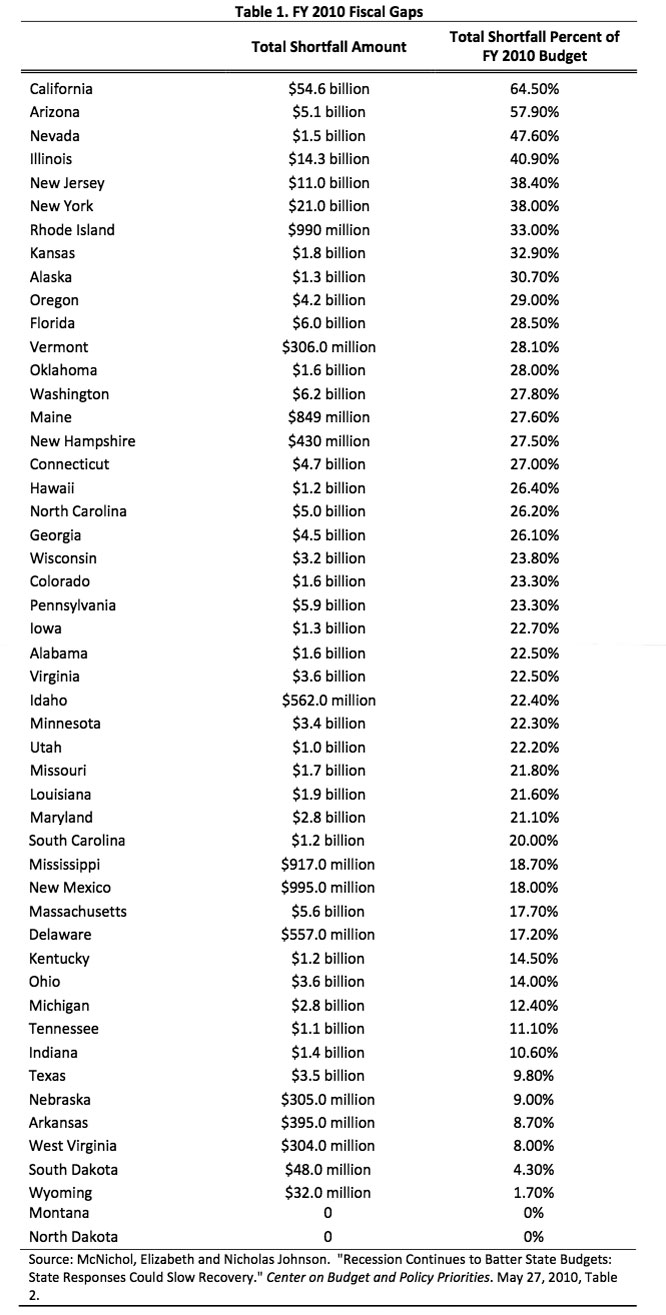
According to the Center on Budget and Policy Priorities, 48 states grappled with FY2010 budget gaps that totaled nearly $200 billion.¹¹ Table 1 reports these gaps, in descending order.

What policies and institutions contributed to these budget gaps? To investigate this question, I ran an OLS regression on the FY2010 state budget gaps and included a number of variables that might explain them. The basic regression model is:

(Budget Gap) = β₀ + β₁(Growth in Per Capita Spending)_t + β₂(Spending Share)_t + β₃(Economic Freedom)_t

Table 2 gives a description of each of the components of this equation.¹² For the dependent variable, I use each state's FY2010 budget gap as a share of its FY2010 budget. These data were computed by the Center on Budget and Policy Priorities and are reported in Table 1.

The first independent variable of interest is Growth in Per Capita Spending. For each state, this variable is the ratio of 2007 per capita spending to 1987 per capita spending. I use the growth in government up until the year prior to the recession because nearly every state has reduced spending after the recession and I am interested in the long‐run effect of spending growth on the budget gap, not in the effect of the recession on spending. Theoretically, those state governments that grow faster might be expected to experience larger budget gaps. This is because both revenue volatility and spending growth are driven, at least in part, by the same cause: progressive taxation. Those states with more progressive tax codes tend to experience faster government growth because, over time, both inflation and real economic growth tend to push more and more taxpayers into higher tax brackets and as the proportion of taxpayers in higher tax brackets increases, government revenues increase. For the same reason, states with more progressive tax codes are likely to see their revenues fall off sharply during a recession as taxpayers drop out of higher tax brackets. If this theoretical relationship bears out in practice, the estimated coefficient on this variable, β₁, should be statistically significant and greater than 0.

In addition to changes in spending, a state government's share of total state income might also influence the size of its budget gap. The hypothesized relationship, however, is ambiguous. It may be that larger state governments are able to allocate more resources to the budgeting process, allowing them to more‐accurately match revenues with expenditures, decreasing the budget gap. Or perhaps causality runs in the opposite direction and states with inherently stable revenue growth patterns are able to balance their budgets and spend a larger share of income (it may be that the economic and political costs of government size are smaller when spending patterns are more stable). In either case, we would expect states with larger budgets as a share of income to have smaller budget gaps. But this may not be the complete story. Alternatively, large state governments may increase state economic volatility and, through that channel, increase the size of the budget gap.¹³ To better understand this relationship, I include a measure of each state's pre‐recession (2007) spending as a share of its total state income.¹⁴ The expected sign on the estimated coefficient on this variable, β₂, is ambiguous; it depends on which of these forces dominates.

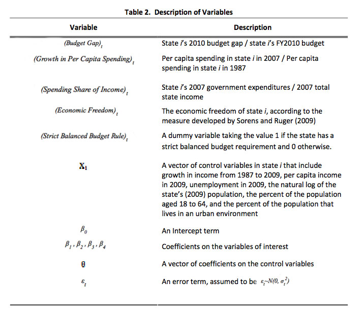
A host of other state policies from labor policy to price regulation to licensing may impact economic growth and the volatility of growth. Through these channels, these policies may also affect the size of a state's budget gap. In order to quantify variation in these sorts of policies, a number of researchers have developed measures of economic freedom—broadly defined as minimal interference with free enterprise.¹⁵ Most of this literature is based on international comparisons, but new research by William Ruger and Jason Sorens extends the study of economic freedom to the state level. Sorens and Ruger gather data on dozens of variables related to state fiscal and regulatory policy. They then aggregate the data to assign each state a score based on the degree to which its policies are consistent with economic freedom.¹⁶ The scores are centered near 0 and range from ‐0.589 (least free) to 0.405 (most free). If economic freedom is associated with economic stability, more economic freedom will lead to smaller state budget gaps. If this is the case, economic freedom might be considered an alternative strategy to achieve fiscal balance. In this case, one would expect the estimated coefficient on Economic Freedom, β₂, to be statistically significant and less than 0.

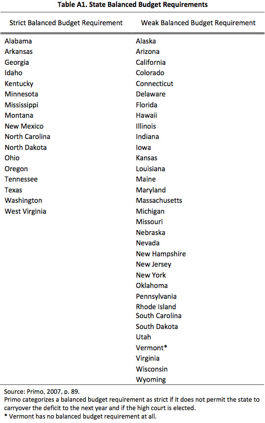
The final variable of interest is a dummy variable, indicating whether or not the state has a strict balanced budget rule. Every state but Vermont has a balanced budget rule, meaning that each of these budget gaps is required by law to be closed. These rules vary considerably in their stringency, however. Some states only require the proposed budget be balanced and not the actual, ex‐post budget. Other states permit a deficit to carry over from one year to the next, while others have a no carryover rule. Lastly, in some states independently‐elected judges evaluate whether or not the legislature has complied with its obligation to balance the budget, while in other states appointed judges decide the question. These institutional differences mean that some states have stricter balanced budget rules than others. Previous research has found that states with stricter balanced budget rules tend to have smaller budget gaps.¹⁷ I rely on Primo's (2007) definition of strict and weak balanced budget rules for the construction of this variable. It takes the value 1 if the state has a no carryover rule and an elected high court—making it a strict balanced budget rule. Otherwise, it takes the value 0—meaning it is a state with either a weak or no balanced budget rule. (Appendix table A1 lists the states according to whether they have strict or weak balanced budget rules). Given previous research, I expect the estimated coefficient on this variable, β₄, to be statistically significant and less than 0.

There are other factors that might impact the size of a state's budget gap. I therefore included a set of control variables that is drawn from the literature on state government spending.¹⁸ These include per capita income in 2009, growth in state income over the period 1987 to 2009, the state's 2009 unemployment rate, the natural logarithm of the state's (2009) population, the percentage of the state population aged 18 to 64 and the percentage of the population that lives in an urban environment. Per capita income and growth in state income are proxies for the demand for public services as well as the size of the potential tax base. In including these variables, I ensure that the Growth in Per Capita Spending and Spending Share variables do not pick up variation in these factors.¹⁹ The unemployment rate is a proxy for potential claims on unemployment insurance and other welfare programs. In including the total population and the percent of the population in an urban environment, I control for economies of scale in the provision of public services. Lastly, young residents and old residents tend to generate the greatest demand for social services. So by including the percentage of the population between 18 and 64, I control for this factor as well.

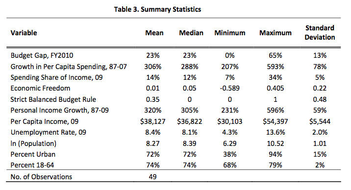
Table 3 reports the summary statistics from the variables used in the regression. As is standard in the literature, I exclude Alaska from the analysis.²⁰ Table 4 reports regression results from three separate ordinary‐least‐squares regressions.

Estimated parameters of the complete model are reported in the second column (Model 1) of Table 4.²¹ P‐values are reported in parentheses.²² In the full model, all of the variables of interest are significant at the 10 percent level, while Economic Freedom and

Strict Balanced Budget Rule

are significant at the 1 percent level.²³ Because some of the control variables failed to obtain statistical significance, I ran additional regressions, keeping only those control variables that obtained marginal or greater significance in the first model. These results are reported in the third and fourth columns (Models 2 and 3). In these models, estimated coefficients on the variables of interest retain their signs and in the case of all but the Strict Balanced Budget Rule, obtain greater statistical significance than in Model 1.

The estimated coefficient on Growth in Per Capita Spending ranges from 0.05 to 0.06. This means that, all else being equal, a 100 percentage‐point increase in the ratio of 2007 per capita spending to 1987 per capita spending is associated with a 5 to 6 percentage point increase in the budget gap. To appreciate the magnitude of this estimate, consider the average state. It had a budget gap of 23% and its 2007 per capita spending level was 306% of its 1987 per capita spending level. What if this state's government had grown slower (say, by one standard deviation)? This would mean that, instead of being 306% of its 1987 level, the state's 2007 per capita spending would have been 228% (=306 ‐ 78) of its 1987 level. The regression model predicts that, all else being equal, this 78 percentage point decrease in the 2007/1987 per capita spending ratio would have produced a budget gap of approximately 19% instead of 23%.²⁴ In other words, its budget gap would have been more than 25% smaller.

How does this compare with the estimated coefficient on Spending Share of Income? This estimate ranges from ‐0.86 to ‐1.5, meaning that all else being equal, states whose expenditure share of income is one point larger than the average tend to have budget gaps that are 0.86 to 1.5 percentage points smaller. Consider, again, the average state. There, spending as a share of total income was 14%. What if this state's expenditures as a share of income had been one standard deviation greater? This would mean that, instead of being 14% of income, 2007 expenditures would have been about 19% (=14 + 5) of income. In this case, the regression model predicts that (all else being equal), this 5 percentage point difference in spending share would have produced a budget gap ranging from 15.5% to 18.7%, instead of 23%.²⁵ It may be that states that have grown accustomed to spending relatively large amounts over the long run develop certain expertise in budgetary planning that allows them to limit the size of their budget gaps. Or perhaps states with stable revenue patterns find it easier to balance their budgets and spend a relatively large share of state income (because, for example, the costs of excessive spending may be smaller when spending is relatively stable). Future research is needed to disentangle these possible explanations.

Taken together, what inferences can we draw from these two results? On the one hand, it seems that states that spend a great deal relative to state income—and have done so for a long time— seem to encounter smaller percentage budget gaps. On the other hand, states whose per capita spending levels grew faster over the preceding decades experienced larger budget gaps. Policy makers, of course, cannot change the past; all they can do is change the future course of policy. And these results suggest that states that increase their per capita expenditures can expect larger budget gaps in the future. They also suggest that, relative to gradual spending accretion, rapid spending growth may make it more difficult to achieve budgetary balance.

Moreover, when we consider this finding in conjunction with that of the tax‐spend literature, we see that an attempt to erase a budget gap by increasing taxes is likely to be self‐defeating in both the short and the long run. That is, the tax‐spend literature seems to indicate that state revenue increases lead to further spending increases in the near term. Moreover, my analysis suggests that state spending increases are associated with larger deficits in the long run. This suggests a vicious cycle from deficits to tax increases, tax increases to spending increases, and spending increases to further deficits.

The results require an important caveat. In this paper, I have not addressed questions of causality. It may be that states that experience persistently large budget gaps are prone to large spending increases.²⁶ To adequately address questions of causality, future research should attempt to instrument for government growth (though this is no simple task).

In addition to restrained spending, the regression results suggest two additional policy options for limiting the size of a state's budget gap. The estimated coefficient on the Economic Freedom variable ranges from ‐24 to ‐31. This means that every 1 point increase in a state's measured economic freedom score is associated with a 24 to 31 percentage point reduction in the state's budget gap. Consider, again, the average state. By Sorens and Ruger's calculations, its economic freedom score is 0.01. A one standard deviation increase in this state's economic freedom (brought about by policies such as lower taxation or less regulation) would give it a score of 0.23 (= 0.01 + 0.23). In this case, the regression predicts that, all else equal, this greater economic freedom would have produced a budget gap ranging from 16% to 18% instead of 23%.²⁷ In other words, a one standard deviation increase in economic freedom is associated with an approximately 30% reduction in the average budget gap.

Another policy option is the adoption of a strict balanced budget rule. It seems that when state legislators constrain themselves by adopting such a rule, they end up encountering significantly smaller budget gaps. The model estimates that those states with a strict balanced budget rule encountered budget gaps that were 8 to 10 percentage points smaller than the average. This amounts to a 35 to 45 percent difference.

Section III. Summary and Conclusion

In many ways, 2010 would seem to be the year of the deficit. Overseas, excessive government deficits upset bond markets and threatened the economies of entire nations (Greece, Italy, Portugal, Spain, Ireland, and Hungary to name a few). In the U.S., the current federal deficit grew considerably and federal debt levels are projected to increase several fold in the coming decades. Meanwhile, nearly every state in the union faced an unprecedentedly large FY2010 budget deficit. In the midst of this, budgets have been cut, employees furloughed, and taxes raised.

The economic problems of government debt and deficits are real. But narrow focus on debt and deficits leaves the false impression that government might "solve" the problem simply by raising taxes. This, however, would substitute one bad—excessive government size—for another—excessive government debt. Worse, the tax-spend literature suggests that in most states, the spending level adjusts to the funds available. This means that tax increases are likely to lead to future spending increases, undoing the deficit‐reducing effect of the initial tax increase.

In Section III, I presented new data examining the factors that contribute to budget gaps. On the one hand, states whose governments spent a larger share of state income and had done so for a while, experienced smaller deficits in FY2010. For the policy maker contemplating a tax increase to shore up his deficit, however, this should be little comfort. This is because I also found that states whose per capita spending levels increased the most between 1987 and 2007 were likely to face significantly larger FY2010 budget deficits.

I also found that states with greater levels of economic freedom (lower taxation and less regulation) experienced smaller FY2010 budget gaps. Using data developed by Sorens and Ruger, I found that a state could cut its deficit by one quarter by increasing its economic freedom score by one standard deviation. Given the large body of literature establishing a link between economic freedom and economic prosperity, economic freedom would seem to be a superior policy strategy for dealing with budget deficits. Lastly, those states that bind themselves with strict balanced budget requirements seemed to encounter smaller budget gaps. Taken together, the results suggest that spending restraint, economic freedom, and strict balanced budget requirements can help states avoid future budget gaps.

Endnotes

1. Alex Johns provided superb research assistance on this paper. I thank Tyler Cowen, Eileen Norcross, Thomas Stratmann, Tate Watkins, and Richard Williams for helpful comments on earlier drafts. I alone am responsible for errors that remain.

2. McNichol and Johnson, 2010.

3. Michael Powell, 2010.

4. U.S. Departmenty of the Treasury and Bureau of Economic Analysis. For the long-term projections, see the Congressional Budget Office’s Alternative Fiscal Scenario in the Long-Term Budget Outlook, 2009.

5. Rauh, 2010.

6. Norcross and Biggs, 2010.

7. Office of Management and Budget.

8. McNichol and Johnson, 2010.

9. Reinhart and Rogoff, 2010.

10. Payne’s research has recently been corroborated by Westerlund, Mahdavi, and Firoozi (2009). The reader is cautioned against extrapolating Payne’s results to the federal level. There, because it is possible for the government to run persistent deficits, voters may suffer from fiscal illusion. In this case, tax increases may actually force voters to come to terms with the cost of government and therefore to demand spending decreases. See Andrew Young (2009) for this perspective. In states where fiscal illusion is more likely (perhaps because the balanced budget rule permits a carryover), one might not expect Payne’s results to hold.

11. McNichol and Johnson, 2010.

12. Budget gap data come from the Center on Budget and Policy Priorities, 2010. Expenditure data are from the National Association of State Budget Officers (1989 and 2009). Economic Freedom scores are from Ruger and Sorens, 2009. The strict balanced budget rule dummy is taken from Primo, 2007. State unemployment rates are from the Bureau of Labor Statistics. All other data are from the Census.

13. See Crain, 2003, for an analysis of state economic volatility.

14. As an alternative to this variable, I also ran the regression using 2007 spending per capita. I obtained similar results.

15. A host of studies have found that economic freedom is positively related to a number of desirable outcomes, most-notably economic growth. For a survey of the literature, see Doucouliagos and Ulubasoglu, 2006. They report (p. 78) that, “regardless of the sample of countries, the measure of economic freedom and the level of aggregation, there is a solid finding of a direct positive association between economic freedom and growth.”

16. Sorens and Ruger also gather data on personal freedom. Given the focus of this paper, however, I only use their economic freedom data.

17. See, for example, Bohn and Inman (1996).

18. See, for example, Crain (2003); Crain and Crain (1998); Bohn and Inman (1996); Matsusaka and Gilligan (1995); Poterba (1994); and Alt and Lowry (1994). My discussion of the control variables draws heavily from Crain (2003).

19. As a robustness check, I also ran the regression using 2007 per capita income and using 1987-2007 to compute the growth in income variable. The results still hold.

20. Alaska’s unusually heavy reliance on energy severance taxes means that it exhibits extremely atypical spending patterns. It is standard practice in cross-state analyses to omit the state for this reason. See Crain, 2003, note 1, p 150.

21. The estimated coefficients reported in Table 4 indicate the (ceteris paribus) relationship between each independent variable and the dependent variable (in this case the Budget Gap). These coefficients represent the slope of the best-fitting line running through a scatter-plot of the independent and dependent variables. The values indicate the rate of change of state budget gaps as each of the other variables change.

22. All regressions were run on Stata/SE 11.0 . The OLS estimates use White’s (1980) heteroscedasticity-consistent standard errors and covariances. All P-values were obtained via a 2-tailed significance test.

23. Statistical significance, indicated here by the P-values, indicates the likelihood that the observed relationship is due to chance. In other words, the P-value 0.041 on the coefficient of Growth in Per Capita Spending in Model 3 indicates that there is a 4 percent probability that the estimated relationship is obtained by chance.

24. 19 = 23 - .05*78

25. 15.5 = 23 - 1.5*5 and 18.7 = 23 - .86*5

26. Crain (2003) posited that revenue volatility might lead to more spending.

27. 16.2 = 23 - 31*0.22 and 17.7 = 23 - 24*0.22

Bibliography

Alt, James, and Robert Lowry. "Divided Government, Fiscal Institutions, and Budget Deficits: Evidence from the States." The American Political Science Review 88, no. 4 (1994): 811-828.

Bartik, Timothy. "Jobs, Productivity, and Local Economic Development: What Implications Does Economic Research Have For the Role of Government." National Tax Journal 47 (1994): 847-862.

—. "Taxes and Local Economic Development: What Do We Know and What Can We Know?" Proceedings of the Eighty-Seventh Annual Conference on Taxation. Charleston, SC: National Tax Association-Tax Institute of America, 1994. 102-206.

Bohn, Henning, and Robert Inman. "Balanced Budget Rules and Public Deficits: Evidence from the U.S. States." Carnegie-Rochester Conference Series on Public Policy 45 (1996): 13-76.

Buchanan, James, and Richard Wagner. Democracy in Deficit. New York: Academic Press, 1977.

Buchanan, James, and Richard Wagner. "Dialogues Concerning Fiscal Religion." Journal of Monetary Economics, 1978.

Bureau of Labor Statistics. REGIONAL AND STATE UNEMPLOYMENT -- 2009 ANNUAL AVERAGES. March 3, 2010. http://www.bls.gov/news.release/srgune.htm (accessed July 1, 2010).

Congressional Budget Office. "Long-Term Budget Outlook." Washington, D.C., 2009.

Crain, Mark. Volatile States: Institutions, Policy, and the Performance of American State Economies. Ann Arbor, MI: University of Michigan Press, 2003.

Crain, Mark, and Nicole Crain. "Fiscal Consequences of Budget Baselines." Journal of Public Economics 67, no. 3 (1998): 421-36.

Doucouliagos, Chris, and Mehmet Ali Ulubasoglu. "Economic Freedom and Economic Growth: Does Specification Make a Difference?" European Journal of Political Economy 22 (2006): 60– 81.

Friedman, Milton. "The Limitations of Tax Limitation." Policy Review, 1978: 7-14.

Matsusaka, John, and Thomas Gilligan. "Deviations from Constituent Interests: The Role of Legislative Structure and Political Parties in the States." Economic Inquiry 33 (1995): 383-401.

McNichol, Elizabeth, and Nicholas Johnson. Recession Continues to Batter State Budgets; State Responses Could Slow Recovery. Washington, D.C.: Center on Budget and Policy Priorities, 2010.

National Association of State Budget Officers. "State Expenditure Report." Washington, D.C., 2009.

National Association of State Budget Officers. "State Expenditure Report." Washington, D.C., 1989.

National Governors Association and National Association of State Budget Officers. "The Fiscal Survey of States." Washington, D.C. , 2010.

Norcross, Eileen, and Andrew Biggs. "The Crisis in Public Sector Pension Plans: A Blueprint for Reform in New Jersey." Mercatus Center Working Paper, June 2010.

Office of Management and Budget. "Table 1.2. Summary of Receipts, Outlays and Surpluses or Deficit as Percentages of GDP: 1930-2015." Washington, DC, 2010.

Payne, James. "A Survey of the International Empirical Evidence on the Tax-Spend Debate." Public Finance Review 31 (2003).

Payne, James. "The Tax-Spend Debate: Time Series Evidence from State Budgets." Public Choice 95, no. 3 (1998): 307-320.

Poterba, James. "State Responses to Fiscal Crises: The Effects of Budgetary Institutions and Politics." The Journal of Political Economy 102 (1994): 799-821.

Powell, Michael. "Illinois Stops Paying Its Bills, but Can't Stop Digging Hole." The New York Times, July 3, 2010: A1.

Primo, David. Rules and Restraint: Government Spending and the Design of Institutions. Chicago, IL: University of Chicago Press, 2007.

Rauh, Jonathan. "Are State Public Pensions Sustainable?" Train Wreck: A Conference on America's Looming Fiscal Crisis. Los Angeles, CA: Urban-Brookings Tax Policy Center/USC-Caltech Center for the Study of Law and Politics, 2010.

Reinhart, Carmen, and Kenneth Rogoff. "Growth in a Time of Debt." American Economic Review Papers and Proceedings. 2010.

Ruger, William, and Jason Sorens. Freedom in the 50 States: An Index of Personal and Economic Freedom. Arlington, VA: Mercatus Center, 2009.

U.S. Bureau of Economic Analysis. National Economic Accounts. 2010. http://www.bea.gov/national/index.htm#gdp (accessed July 10, 2010).

U.S. Census Bureau. "Statistical Abstract of the United States: 2010." Washington, D.C., 2009.

U.S. Departmenty of the Treasury. Debt to the Penny. http://www.treasurydirect.gov/NP/BPDLogin?application=np (accessed July 12, 2010).

Westerlund, Joakim, Saeid Mahdavi, and Fathali Firoozi. "The Tax-Spending Nexus: Evidence from a Panel of US State-Local Governments." University of Gothenburg Working Paper in Economics No. 378, 2009.

White, Halbert. "A Heteroskedasticity-Consistent Covariance Matrix Estimator and a Direct Test for Heteroskedasticity." Econometrica 48, no. 4 (1980): 817-838.

Young, Andrew. "Tax-Spend or Fiscal Illusion?" Cato Journal 29, no. 3 (2009).

Appendix