What Would Milton Friedman Say about the Recent Surge in Money Growth?

This policy brief is part of a Mercatus Symposium titled “What Would Milton Friedman Say?” The symposium explores what the late Nobel laureate, economist Milton Friedman, might say about monetary policy today, as the Federal Reserve grapples with increasing inflation in the wake of the COVID-19 pandemic.

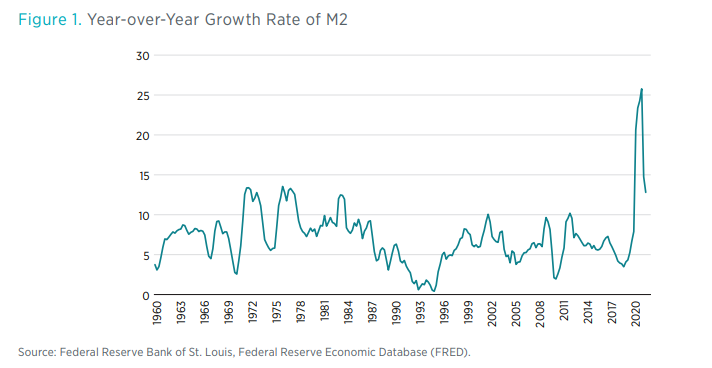
The M2 money supply grew at annualized rates exceeding 20 percent throughout much of 2020. Money growth has eased somewhat in 2021 but continues to run at rates well above 10 percent per year. As a result, M2 stands more than 36 percent higher today than it did at the end of 2019. Figure 1 confirms that nothing like this has been seen before, at least not since 1960 and not even during the high-inflation years of the 1970s.

These numbers, by themselves, raise the strong possibility that we have entered a new and quite remarkable era in US monetary history. Does the past serve as any guide to what this new era might eventually bring? What would Milton Friedman say?

Although Friedman’s contributions range broadly across many areas of economics, he is best known for his research on monetary history, conducted jointly with Anna J. Schwartz. Friedman and Schwartz’s Monetary History of the United States, particularly its chapter on the Great Depression of 1929–1933, remains one of his most famous works. That volume uses a narrative approach to link fluctuations in the money supply to subsequent movements in output, employment, and inflation. It thereby identifies monetary instability as the principal driving force behind instability in the economy as a whole.

Despite Friedman’s fame and influence, however, academic economists and central bankers rarely think, today, about monetary policy in terms of its effects on money growth. They focus instead on interest rates. Their emphasis on interest rates reflects, partly, a professional consensus that the statistical links between measures of the money supply and other key macroeconomic variables weakened in the late 1980s and early 1990s. In fact, Friedman was well aware that patterns in more recent data differ from those that he found earlier in his historical analyses.

Nevertheless, Friedman surely would be alarmed by the recent surge in M2 growth. One can, in fact, use insights gleaned from Friedman’s research to see that although the statistical relationships between money growth, real GDP growth, and inflation may have weakened somewhat in recent decades, they have in no way disappeared. Thus, rapid M2 growth serves as a warning sign. Unless the Federal Reserve acts soon and decisively to recalibrate its monetary policy strategy, higher inflation will quite likely persist.

MONEY, BUSINESS CYCLES, AND INFLATION

In their Monetary History and in related statistical work, Friedman and Schwartz find strong links between money growth and business cycles in data extending back to 1867 and running through 1960.4 In those data, money growth consistently peaks just before output and employment reach their own cyclical peaks, and money growth troughs just before output and employment hit their cyclical troughs. Moreover, moderate declines in money growth presage mild economic recessions, while deeper monetary contractions portend more severe economic depressions.

In documenting these general facts, Friedman and Schwartz reshaped economists’ understanding of the Great Depression. Whereas previously, scholars believed that the Federal Reserve had done all it could to mitigate the effects of the Great Depression, Friedman and Schwartz showed the Fed was largely to blame for its length and depth. According to Friedman and Schwartz, the initial economic downturn following the stock market crash of 1929 would have been severe in any case. However, nothing like the Great Depression that eventually ensued would have been possible without years of relentlessly tight monetary policy, reflected in a prolonged decline in the M2 money stock. Here, it is most helpful to review Friedman and Schwartz’s own words:

"Monetary behavior during the contraction itself is even more striking. From the cyclical peak in August 1929 to the cyclical trough in March 1933, the stock of money fell by over a third. This is more than triple the largest preceding declines recorded in our series. . . ."

"The monetary collapse was not the inescapable consequence of other forces, but rather a largely independent factor which exerted a powerful influence on the course of events. The failure of the Federal Reserve to prevent the collapse reflected not the impotence of monetary policy but rather the particular policies followed by the monetary authorities. . . ."

"The contraction is in fact a tragic testimonial to the importance of monetary forces. . . . For it is true also . . . that dif­ferent and feasible actions by the monetary authorities could have prevented the decline in the stock of money—indeed, could have produced almost any desired increase in the money stock. . . . Prevention or moderation of the decline in the stock of money, let alone the substitution of monetary expansion, would have reduced the contraction’s severity and almost certainly its duration. The contraction might still have been relatively severe. But it is hardly conceivable that money income could have declined by over one-half and prices by over one-third in the course of four years if there had been no decline in the stock of money."

Naturally, after World War II, Friedman’s attention shifted away from the role that monetary contraction played in driving deflation and depression to the role that excessive money growth played in generating a recurrent, inflationary boom-bust cycle. His critique begins in chapter 10 of the Monetary History, on “World War II Inflation, September 1939–August 1948,” an episode also discussed by Michael D. Bordo and Mickey D. Levy.

M2 growth accelerated during World War II, as the Federal Reserve concentrated on keeping interest rates low to support government borrowing. During the war itself, measured inflation remained subdued, reflecting the imposition of wage and price controls together with increased household saving in response to a shortage of durable goods. After the war, however, controls were lifted and pent-up spending power was released, leading to two years of double-digit inflation in 1946 and 1947. This historical experience takes on new relevance today, of course, as M2 growth has surged even as business shutdowns and disrupted supply chains have led to shortages of many consumer durable goods.

Friedman and Schwartz’s Monetary History concludes before US inflation rose more persistently during the 1970s. Instead, Friedman’s views on the sources of the “Great Inflation” and the chronic economic instability that accompanied it can be found in a series of essays published later. An October 1977 column from Newsweek magazine, for example, presages today’s debates by focusing on whether inflation is “transitory or persistent.” There, Friedman writes:

"There is one and only one basic cause of inflation: too high a rate of growth in the quantity of money—too much money chasing the available supply of goods and services. These days, that cause is produced in Washington, proximately, by the Federal Reserve System, which determines what happens to the quantity of money; ultimately, by the political and other pressures impinging on the System, of which the most important are the pressures to create money in order to pay for exploding Federal spending and in order to promote the goal of “full employment.” All other alleged causes of inflation—trade union intransigence, greedy business corporations, spend-thrift consumers, bad crops, harsh winters, OPEC [Organization of Petroleum Exporting Countries] cartels and so on—are either consequences of inflation, or excuses by Washington, or sources of temporary blips of inflation."

Then, in a lecture published by the Bank of Japan, Friedman describes in more detail how the Fed’s practice of conducting monetary policy by managing interest rates contributed to both inflation and economic instability:

"In practice, the Fed continued to target interest rates, specifically the Federal funds rate, rather than monetary aggregates, and continued to adjust its interest rate targets only slowly and belatedly to changing market pressure. The result was that the monetary aggregates tended on average to rise excessively, contributing to inflation. However, from time to time, the Fed was too slow in lowering, rather than in raising the Federal funds rate. The result was sharp deceleration in the monetary aggregates, and an economic recession."

Finally, Friedman sums up concisely the conclusions of his lifetime’s work studying the Fed:

"To summarize this 69-year record: two major wartime inflations; two major depressions; a banking panic far more severe than was ever experienced before the Federal Reserve System was established; a succession of booms and recessions; a post–World War II roller coaster marked by accelerating inflation and terminating in four years of unusual instability—the whole relieved by relative stability and prosperity during the two decades after the Korean War."

"Granted, the Fed alone is not to blame for this dismal record. Yet it is—to put it mildly—hardly an impressive performance compared either to our nation’s experience before the Federal Reserve System was established or to the record of some other nations with a different monetary structure."

Both the substance and the tone of these comments leave no doubt that Friedman would be quite concerned by the recent surge in money growth as a source of persistent inflation and, possibly, the cause of a future recession if the Fed waits too long to correct for it and must then adjust its policies more vigorously later on. There is, however, a significant complication that Friedman would have to address in making his case for the importance of money growth today.

“I’M BAFFLED”

Sometime in the mid to late 1980s, the strong correlations between money growth, output, employment, and inflation that Friedman and Schwartz first uncovered started to weaken. By the early 1990s, many economists had concluded that short-term interest rates, such as the federal funds rate, serve more reliably to indicate the stance of monetary policy and, hence, bear a closer relationship to key macroeconomic variables.

Two articles published in the American Economic Review—the first by Ben S. Bernanke and Alan S. Blinder and the second by Benjamin M. Friedman and Kenneth N. Kuttner—proved highly influential in shaping this new consensus among academic economists. Meanwhile, Federal Reserve officials and policy advisers acknowledge that the Fed placed increasing emphasis on managing the federal funds rate and paid correspondingly less attention to the monetary aggregates throughout the 1990s. In September 1998, the Federal Open Market Committee (FOMC) initiated the practice, which it continues to this day, of announcing an explicit target for the federal funds rate immediately after each meeting. And in June 2000, the FOMC stopped announcing target ranges for money growth.

Eventually, even Milton Friedman had to confront these new realities. In an interview with John Taylor published in 2001, Friedman presented a graph comparing year-over-year growth rates in real M2 and real GDP from 1960 through 1999. Figure 2 reproduces and extends Friedman’s chart so that it runs through 2021, quarter 3. Both Friedman’s original graph and the update here show real M2 and real GDP moving closely together from 1960 through the mid to late 1980s. Thereafter, the relation breaks down.

Table 1 quantifies this shift. Before 1990, the correlation between the two series is 0.56; since then, it is –0.43. Combining the first three decades of positive comovement with the last three decades of negative comovement, the correlation for the full sample comes in at virtually zero. In fairness, the most recent observations, reflecting the sharp contraction in real GDP associated with the economic shutdown in March 2020 and the coincident burst in M2 growth, surely reflects the Federal Reserve’s response to an unprecedented crisis. However, even when these observations are excluded, the correlation between real M2 and real GDP growth remains negative, at –0.33, from 1990 through the end of 2019. The equation of exchange reads

MV= PY,

where M is the money supply, V is the velocity of money, P is the aggregate nominal price level, and Y is real GDP. Rewritten as

m + v = p + y,

where lowercase variables denote the growth rates of the corresponding uppercase variables, this equation makes clear that changes in velocity, causing v ≠ 0, will weaken the connections between money growth m, inflation p, and real GDP growth y.

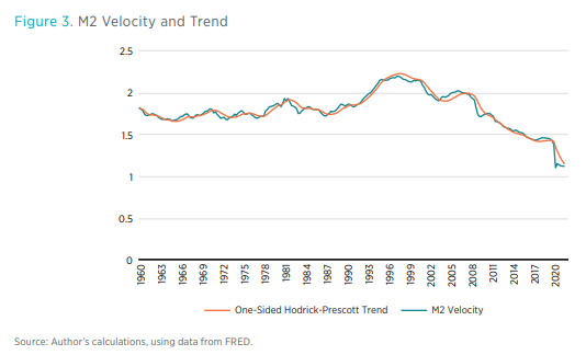
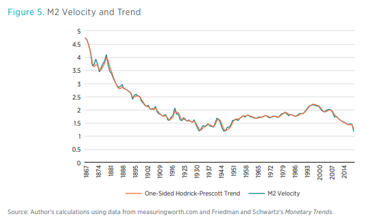
Thus, in a second graph presented to Taylor, Friedman plotted the velocities of M1, M2, and M3 to pinpoint the precise timing of the break. Figure 3 reproduces and updates Friedman’s chart, focusing on M2 velocity. Again, both Friedman’s graph and the update presented here show that the velocity of M2, which had remained remarkably stable throughout the 1960s, 1970s, and 1980s, moved unexpectedly higher in the early 1990s. The extended graph here reveals that in addition, the earlier stability in M2 velocity never returned. After rising from 1992 through 1995, M2 velocity reversed course and has relentlessly declined ever since.

These post-1990 movements in velocity need not be viewed as completely random, divorced from economic fundamentals.19 Nevertheless, they clearly underlie the shift in money-output correlations, from positive to negative, seen in figure 2. In his interview with Taylor, Friedman confessed, “I’m baffled."

And, yet, insights from Friedman’s earlier work can help reconcile the recent data with his preferred quantity-theoretic approach to predicting and understanding the effects that monetary policy in general and money growth in particular have on the economy.

THE QUANTITY THEORY REVISITED

Long before his interview with Taylor, Friedman provided his own “restatement” of the quantity theory of money. Friedman begins with a summary: “The quantity theory is in the first instance a theory of the demand for money.” Later, he elaborates: 

The quantity theorist accepts the empirical hypothesis that the demand for money is highly stable. . . .This hypothesis needs to be hedged on both sides. On the one side, the quantity theorist need not, and generally does not, mean that the real quantity of money demanded per unit of output, or the velocity of circulation of money, is to be regarded as numerically constant over time. . . . On the other side, the quantity theorist must sharply limit, and be prepared to specify explicitly, the variables that it is empirically important to include in the function. For to expand the number of variables regarded as significant is to empty the hypothesis of its empirical content; there is indeed little difference between asserting that the demand for money is highly unstable and asserting that it is a perfectly stable function of an infinitely large number of variables.

To illuminate further both “sides” of his hypothesis, Friedman reexpresses the equation of exchange (1) by depicting velocity V not as a constant but instead as a function of a small set of variables:

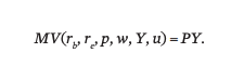
In (3) , r_b and re are the expected returns on bonds and equities, w is the ratio of capital to labor income, and as before, p and Y are the rate of inflation and the level of real income. According to Friedman, these are the most important variables shaping the portfolio allocation problems faced by households and firms and thereby affect the demand for money as one of many financial assets. Meanwhile, u is a composite index of geographic mobility and economic uncertainty that, Friedman hypothesizes, may also affect money demand.26 Thus, in (3), nominal GDP PY is determined through the interaction between changes in the nominal supply of money M and the demand for real money represented by the function V.

In the edited volume that contains it, Friedman’s essay is followed by a series of studies—by Phillip Cagan, John J. Klein, Eugene M. Lerner, and Richard T. Selden—that provide empirical evidence to support the quantity theory. David E. W. Laidler surveys the voluminous literature that appeared as many other economists continued to pursue this research agenda throughout the decades that followed, presenting estimates and tests of equations linking real money demand to a small number of fundamental determinants. And although the same shifts in velocity shown in figure 3 led to a slowdown in research on money demand in the 1990s, work along these lines continues to this day.

Michael T. Belongia and Peter N. Ireland take a slightly dif­ferent approach to the empirical implementation of the quantity-theoretic ideas expressed by Friedman through (3). Observing that the determinants of money demand identified by Friedman and throughout the subsequent literature are likely to evolve only slowly over time, Belongia and Ireland rewrite the equation of
exchange (1) as

where the first equality defines a shift-adjusted measure of the money stock M that corrects for long-run movements in velocity captured by the new variable V*.  Thus, in (4), V! becomes the deviation of actual velocity V from its long-run level V*.

By replacing (3) with (4) as the equation that gives the quantity theory its empirical content, Belongia and Ireland accept Friedman’s view that the quantity theory does not require velocity to be numerically constant. At the same time, however, Belongia and Ireland must also concede that for (4) to serve as a practical guide to monetary policymaking and monetary policy evaluation, the long-run level of velocity V* must be estimated in real time—that is, without the use of data that only become available after policy decisions affecting the current money supply M have been made. Moreover, they must hope that unpredictable changes in velocity V away from the estimated long run level V* remain small enough that stability in V will provide, via (4), a tighter statistical connection between growth in shift-adjustment money M and growth in nominal GDP PY.

With these goals in mind, Belongia and Ireland produce estimates of V* using the one-sided version of the Hodrick-Prescott filter described by James H. Stock and Mark W. Watson. Crucially, the “one-sided” nature of this statistical procedure means that the time-varying estimate of V* is updated based on only current and past—but not future—data on velocity itself. Thus, provided the determinants that enter Friedman’s velocity function do move slowly, the one-sided filter provides an attractive alternative to estimating a specific, multivariate regression for money demand and dealing with the parameter instabilities that inevitably seem to plague such models.

Figure 3 confirms that, in fact, the one-sided estimate of trend velocity V* tracks quite closely movements in actual velocity V over the entire 1960:1–2020:3 sample of quarterly data. Movements in the estimated trend do tend to lag movements in velocity itself, reflecting, of course, the one-sided nature of the time-series filter. However, because velocity drifts up and down very gradually and does not display large quarter-to-quarter movements, the deviations of V from V* are small. Thus, as hoped for earlier, V in (4) remains stable.

Figure 4 redraws figure 2, with growth in real shift-adjusted M2 replacing growth in real M2 itself. Before 1990, the picture looks much the same as it did before, reflecting the underlying stability of M2 velocity itself over that first part of the sample. After 1990, however, the graph shows a much tighter relationship between real money and output growth. Table 1, again, helps to quantify. When shift-adjusted M2 replaces M2, the correlation between real money and output growth 

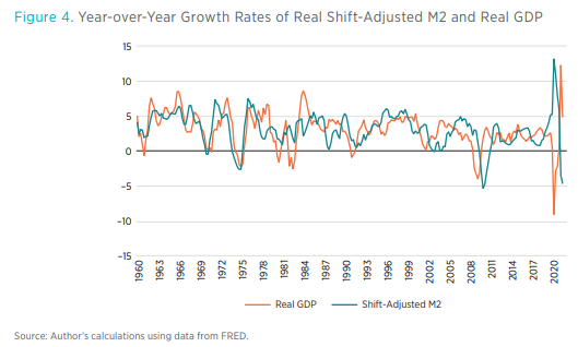
computed with data from 1990 through 2019 flips in sign: from −0.33 in figure 2 to 0.26 in figure 4. The correlation computed with all the pre-2020 data increases from 0.27 to 0.46.

It is interesting to use Friedman and Schwartz’s long historical series on M2 to extend the analysis back further, just as they did.35 Figure 5 reveals that M2 velocity declined persistently from 1867 through the end of World War II. This graph serves to highlight, therefore, that the period of stable M2 velocity from 1960 through 1990 is the exception, not the rule. The graph also shows, 

however, that movements in M2 velocity remain smooth enough to be tracked quite well and in real-time using the one-sided Hodrick-Prescott filter.

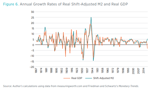
Figure 6 then shows a remarkably tight relationship between real shift-adjusted M2 growth and real GDP growth extending from 1867 through the present. Clearly visible in the graph is the deep monetary contraction that lies at the heart of Friedman and Schwartz’s explanation of the Great Depression. Table 1 summarizes that the correlation between real shift-adjusted M2 growth and real GDP growth exceeds 0.80 over sample periods starting in 1867 and ending in 1989, 2019, or 2020. Focusing narrowly on the episode from 1990 through 2019, the correlation, at 0.56, remains sizable.

Altogether, these findings should reassure quantity theorists who might otherwise struggle, as Friedman himself did in his interview with Taylor, to interpret the recent behavior of M2. Although it is true that the extremely tight links between money and the business cycle loosen somewhat, they remain evident in the post-1990 period provided allowance is made for slow-moving trends in velocity. And they appear larger still, when the quarterly data originally presented by Friedman to Taylor are replaced by annual data. This makes sense, as annual averaging smooths out quarter-to-quarter noise in measured GDP so as to focus on intermediate-term trends, which are more likely driven by macroeconomic fundamentals, including Federal Reserve monetary policy.

It is also interesting to use the quantity-theoretic approach embodied in (4) to assess the strength and stability of links between shift-adjusted nominal money growth and inflation, an important issue that Friedman did not discuss in his interview with Taylor. Figure 7 compares these series using the long annual time series, running back to 1867, originally provided by Friedman and Schwartz but extended through the present. The graph shows clearly that episodes of major inflation—most significantly those during World War II and the 1970s—are accompanied by rapid growth in the shift-adjusted money supply. And the graph shows, just as clearly, episodes of disinflation or even outright deflation—following World War I, during the Great Depression, in the early 1980s, and for a brief period during the financial crisis of 2008–2009—coincide with periods of decelerating money growth or outright monetary contraction.

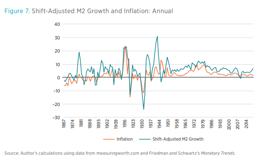
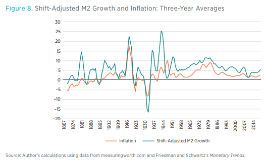
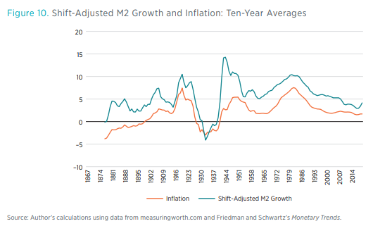
Figure 7 also shows that, even more so than real GDP growth, measured inflation exhibits yearto-year volatility that is unrelated to intermediate and longer-run monetary trends. Robert Lucas demonstrates that quantity-theoretic links between money growth and inflation are revealed much more clearly when multiyear moving averages of both series are compared. Following this approach, figures 8–10 plot three-, five-, and ten-year moving averages of shift-adjusted nominal M2 growth and inflation.

Most strikingly, figure 10 renders visible the various eras of monetary policy successes and failures mentioned in the passage quoted above from Friedman: rapid money growth and inflation during both world wars, monetary contraction and with severe and persistent deflation during the Great Depression, accelerating money growth and inflation again during the 1970s, and more encouragingly, two periods of stable money growth and inflation following the Korean War and, again, starting in the mid-1980s.

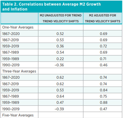
Table 2 confirms that the measured correlations between money growth and inflation become stronger, first, when slow-moving trends in velocity are accounted for and especially when the data are averaged over longer horizons. Most notably, the correlation between ten-year moving averages of shift-adjusted money growth and inflation over the period from 1867 through 1989 is 0.85.

And even focusing on the most recent decades, from 1990 through 2019, the correlation between those series is 0.49. Also visible in figures 7–10 is the sharp acceleration in money growth in 2020. The message from this analysis, based on Friedman’s monetary economics, is that the recent bulge in M2, if not reversed, will soon fuel higher inflation.

WHAT HAPPENS NEXT?

As revealed by Friedman’s 1977 Newsweek column, today’s debates over whether inflation will prove “transitory or persistent” echo strongly similar debates over the role that Federal Reserve policy played in driving inflation higher during the 1970s. Friedman’s position in that debate was unequivocal. The words he used back then are the ones he would most likely use today. To repeat: “There is one and only one basic cause of inflation: too high a rate of growth in the quantity of money.”

In Friedman’s absence, Robert Hetzel, and Peter N. Ireland and Mickey D. Levy elaborate on this position by emphasizing that “what happens next” depends crucially on what the Federal Reserve does next. As noted above, FOMC members have not systematically followed movements in M2 or any other measure of the money supply in many years. And it is unlikely that they will change their approach to monetary policymaking by paying more attention to money anytime soon. Still, one can ask how the Fed’s current strategic framework, based on a combination of large-scale asset purchases (or “quantitative easing”) and federal funds rate management, determines the behavior of the M2 money supply and thereby influences economic growth and inflation.

As the US economy continues to recover from the March 2020 shutdowns, consumer and business confidence will continue to improve, risk aversion will ease, and the demand for precautionary savings will diminish. What Friedman called the “natural” rate of interest will rise.40 If against this backdrop the FOMC is willing to wind down its asset purchase programs rapidly and to begin raising its target for the federal funds rate in lockstep with the rising natural rate, households and firms will have the incentive to use their stocks of liquid assets—reflected in the now-elevated level of M2—to save and pay down debt. As they do, bank deposits will be extinguished. The bulge in real M2 from 2020 and 2021 will dissipate as the increase in nominal M2 reverses itself. Inflation will fall back to lower, more acceptable levels.

Suppose, on the other hand, the FOMC moves too slowly to end quantitative easing. Michael T. Belongia and Peter N. Ireland show that just like more traditional open market operations—also purchases of government bonds with newly created bank reserves—large-scale asset purchases generate faster growth in M2. Thus, in this alternative scenario, rapid growth in nominal M2 will not cease.

Suppose also that meanwhile, the FOMC persists in holding the federal funds rate target below the rising natural rate. This leaves households and firms ready to spend. The recent rise in real M2 will still reverse itself but through a large and persistent rise in the nominal price level—that is, through inflation. And the longer the FOMC waits before raising rates, the greater becomes the risk that more dramatic policy actions—in the form of even steeper and more abrupt interest rate increases—will be needed to bring inflation back down. The boom-bust pattern of the 1970s will reappear, with high and volatile inflation accompanied by another recession.

So what would Milton Friedman say about the recent surge in M2 growth? That it signals strongly that the Federal Reserve needs to adjust its policies sooner, rather than later, to avoid persistently higher inflation and, possibly, another recession to correct for it later.

Citations and endnotes are not included in the web version of this product. For complete citations and endnotes, please refer to the downloadable PDF at the top of the webpage.