Accounting for the Opportunity Cost of Capital in Cost-Benefit Analysis: Public Interest Comment on the Marginal Excess Tax Burden as a Potential Cost under Executive Order 13771

This comment presents a framework for how the Office of Management and Budget (OMB) should be thinking about the opportunity cost of capital in cost-benefit analysis (CBA). The comment begins by explaining why improvements in CBA are needed at federal agencies. Next, it discusses how to account for displaced investment in CBA using the shadow price of capital (SPC) method, which is technically the appropriate way to account for the opportunity cost of capital in CBA. It then explains why the Executive Order (EO) 13771 accounting statements, where only financial impacts are considered, are a potential improvement over analysis generally produced under EO 12866. Finally, it make several recommendations for improving the EO 13771 accounting statements.

The Shadow Price of Investment

A common mistake made by regulatory agencies in their CBA is to treat all benefits and costs as if they are growing at the same rate, when in fact different benefits and costs evolve differently through time depending on whether they come in the form of investment or consumption. This mistake is especially a concern for social regulations targeting risks to health, safety, and the environment, which often have a heterogeneous mix of benefits.

OMB Circular A-4 notes that the “analytically preferred” method of accounting for the opportunity cost of capital in CBA is to apply a shadow price to investment. The SPC method was developed by economists Stephen Marglin, David Bradford, and Robert Lind, among others. It works by multiplying a particular amount of investment that is generated or displaced by government projects by a conversion factor (the SPC) in order to convert the investment into its consumption equivalent.

The SPC method works very similarly in nature to pricing a stock or a bond, in that a capital asset can be priced by valuing the stream of income that it generates. With capital, however, rather than a dividend or a coupon payment stream, the relevant income stream is the stream of consumption that the capital asset generates.

One begins with the simple case where all of the returns to capital are consumed each period. In this scenario, the principal value of the capital wealth base never grows, and so the capital asset simply produces an infinite stream of equal consumption payments, which can be valued according to the formula

This states that the SPC is equal to the return on investment (ROI), which is the marginal social rate of return to capital net of depreciation, divided by the social rate of time preference (SRTP).

In this simple case, capital is valued like a perpetuity in financial analysis. However, the assumption of no reinvestment is an extreme one, and in the more likely case that some of the return to capital is reinvested each period while the remaining portion is consumed, the SPC equation becomes

Here, f is the fraction of the return that is invested each period, so (1 − f) × ROI is what is consumed in the initial period out of the first-period ROI. The consumption stream that capital generates grows at a rate of f × ROI each period, which for simplicity I will denote as g going forward. The consumption stream is then discounted each period at the SRTP, which for shorthand I will denote as r*. Finally, the stream of consumption is aggregated across time periods, and the resulting SPC conversion factor can then be multiplied by investment flows in CBA.

The variable r* is a special case of a more general parameter, r, the risk-free market interest rate. The market interest rate will only equal the SRTP, or r*, in the special case where the economy is operating along an optimal growth path that is free of distortions that result from taxes and market imperfections, such as externalities. While r* depends in part on one’s normative values about how much to discount the future, for the sake of mathematical convenience, many economists simply assume r* > g, which is a convergence condition akin to the transversality condition from growth theory. If one takes the limit of equation 2 as the time horizon extends to infinity, then equation 2 simplifies to

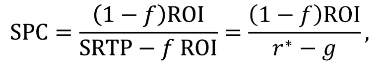
assuming that the transversality condition holds (or that r* = g). This equation can be found in some academic papers written by supporters of the SPC method, and it is similar in nature to how a stock with a growing dividend would be priced. Equation 3 is a shorthand version of equation 2 that can be used when the SPC converges to a finite number. In cases where the transversality condition does not hold because r* < g, equation 2 is the more general form that intuitively shows why the SPC is unbounded when r* is less than g.

The Transversality Condition

It is not sufficient to simply assume that this variant of the transversality condition holds for the sake of mathematical convenience, because a very different set of policy prescriptions will be in order depending on whether the condition holds or not. The transversaility condition is not even a particularly realistic assumption in economic growth models. It represents an assumption that the representative household or agent—which in the Ramsey growth model constitutes something like society as a whole—will exhaust all wealth at the end of the planning horizon. However, the history of human civilization is one where per capita wealth continues to rise over time.

In general, society will want to invest up until the point where the net marginal social rate of return to capital net of depreciation, or g, falls to r*. Only when r* = g would society be indifferent between an additional dollar of investment and an additional dollar of consumption. In that case, social utility would be optimized across time (although it may still not be optimized within a time period).

When  r* < g, investing funds is preferable to consuming at the relevant margin, and so society should seek to spur more investment until g falls to r*. By contrast, when r* > g, the opposite is true. Society will want to consume more until g rises to r*, which is a situation akin to “dynamic inefficiency” in economic growth theory. Thus, from a policy perspective, it is a critical question as to which situation is true. In one case, society will want to spur more investment, and in the other case, more consumption. The policy implications could not be more different.

A critical piece of information to answer this question is what r* is; i.e., what is the SRTP? And that question has a relatively simple answer, it turns out, so long as CBA measures Kaldor-Hicks efficiency. A trademark characteristic of Kaldor-Hicks efficiency is that it is insensitive to equity and distributional concerns. In other words, it avoids judgments about the desirability of how wealth is distributed in society and is concerned solely with changes in aggregate wealth induced by a policy, irrespective of distribution.

It turns out that an analysis using any r* other than zero will not be insensitive to distributional concerns, because analysis would weight consumption depending on when it is delivered. The SRTP can be thought of as similar to a distributional weight that is applied within a time period in CBA. Distributional weights are obviously inconsistent with Kaldor-Hicks efficiency, as they weight consumption depending on who receives it. Similarly, any SRTP other than zero is a violation of Kaldor-Hicks efficiency because unequal weights are applied depending on timing. Whether applying distributional weights within a time period or across time, the requirement that analysis be insensitive to distributional concerns is violated with such weights, violating Kaldor-Hicks efficiency.

Only in the special case where r* = g = 0 would the economy be operating along an optimal growth path that could therefore be considered dynamically efficient: zero is the only SRTP that is totally indifferent with respect to distributional concerns, and r* must equal g as a necessary condition of optimization. The situation where r* = g = 0 also has an intuitive meaning in that it corresponds with a rate of economic growth where all investment opportunities have been exhausted. Therefore, an additional dollar of investment yields a rate of return of zero, thereby providing no more wealth than a dollar of consumption. By extension the flow of consumption produced by wealth over time is maximized, a situation akin to the Golden Rule rate of economic growth from growth theory. When this rate of economic growth is achieved—and only when it is achieved—can the economy be considered dynamically efficient.

EO 13771 Accounting Statements

If CBA is to measure allocative efficiency, then r* must be zero. This may seem like a problem, but intuitively all this means is that one dollar of investment is more valuable to society than a dollar of consumption at the relevant margin; it’s a recipe for preferring investment over consumption until the rate of return to capital falls sufficiently such that capital’s rate of return and consumption’s rate of return are identical.

It turns out that setting the social discount rate at zero can make CBA easier to conduct, because the entire practice of monetizing nonmarket goods often becomes unnecessary. Unless consumption streams are compounding at rates of return through time in excess of investment rates of return—something that generally seems unlikely given that utility can’t be invested like money can—all that will matter in the limit are the capital investment streams.

Investment streams in the future can be discounted at a rate of g—their growth rate—to find their present value. The discount rate in this case is not discounting consumption, but instead it acts as a device to project how different investment streams will grow into the future. If a regulation, on balance, increases the discounted present value of investment, then the rule moves the economy closer to dynamic efficiency.

Interestingly, this method is somewhat close to what OMB is already doing in its EO 13771 accounting statements, which focus on financial impacts of regulations. Financial flows can be divided into streams that are consumed and streams that are invested. However, if the same fraction of all cash flows is invested, one can simply discount the cash flows at the corresponding investment growth rate g and not worry too much about how much of the streams is devoted to consumption. The discounted present values of cash flows and investment streams will be proportional to one another.

There are several ways of thinking about how to calculate g, and the calculation may depend on whether one decides to think about the SPC equations from a macroeconomic or a microeconomic perspective. For example, g could be something like 7 percent, which OMB currently claims approximates the marginal rate of return to private capital in the market. If the nation as a whole invests about 20 percent of its income annually and in doing so achieves a 7 percent return on the margin in private markets, the implicit ROI value on the whole stock of the economy’s wealth is something around 35 percent.

On the other hand, it might be more useful to think that ROI is 7 percent, rather than g. In that case, it would not be very useful to multiply 7 percent by 0.2, the fraction of income saved in the United States annually, because one is interested in what fraction of the marginal dollar is likely to be reinvested, as opposed to the average dollar. This marginal value is almost certainly going to be much greater than 0.2, meaning it might be reasonable to think that g lies somewhere between 3 and 6 percent or so. A benefit of this approach is that OMB uses similar rates as its recommended social discount rates. However, OMB should be clear that, in this context, these are investment rates of interest, not the social discount rates use to discount nonpecuniary benefits and costs.

Recommendations

OMB policy under executive orders 13771 and 12866 could be improved in several ways. First, CBA for social regulations is not properly accounting for the opportunity cost of capital, because it doesn’t employ a shadow price. It is also generally not evaluating economic efficiency, because the r* used in those analyses is not zero. OMB should start to enforce the SPC method, so that the opportunity cost of capital can be conducted properly and analysis can move toward measuring something meaningful, such as Kaldor-Hicks efficiency. A basic framework for how to begin to do this is presented in this comment.

Second, EO 13771 accounting statements represent an improvement over CBA practices under EO 12866 generally, especially for social regulations. This is true because those statements focus on investment streams and don’t conflate the different growth rates of heterogeneous benefits and costs.

One issue of concern is that currently OMB calculates costs and cost savings in its EO 13771 annual statements and then converts them into an annualized value. This is misleading because it implies these impacts are not growing over time. It would be preferable to calculate a present value of costs and cost savings, discounted at a rate of g, to account for the fact that costs and cost savings are compounding in value over time. A rate of g of 3 or 7 percent seems reasonable, though other rates could serve as supplements.

Opportunity cost remains an undervalued concept at federal regulatory agencies. But OMB is on the right track with its EO 13771 accounting statements. With a few small tweaks, these statements could potentially improve CBA practices in a fundamental way and constitute a best practice for other agencies to follow.