An Inflation Primer

Inflation is an increase in the general level of prices in an economy. When the inflation rate is positive, the purchasing power of money falls because more money is required to purchase the same basket of goods as time goes on. Although economists disagree about what the optimal inflation rate should be, inflation can be very harmful.

The definition of inflation may seem straightforward, but there are multiple ways of measuring inflation. Also, despite decades of studying inflation, economists still disagree about the causes of inflation, especially when inflation is high such as in today’s environment. Confusion over the meaning and causes of inflation can lead policymakers and the public to misguided conclusions about how to address it. This policy brief provides an overview of inflation measurement and a framework for how to understand inflation’s causes. Although nonmonetary factors can temporarily affect the price level, inflation is ultimately determined by the monetary authority, the Federal Reserve (Fed) in the case of the United States. Inappropriately high inflation is the product of poor monetary policy.

Measuring Inflation

Inflation is measured by the percentage rise of a price index or “basket of goods.” Usually, it is calculated at a year-over-year rate or a month-to-month rate. The two most common price indices in the United States are the Consumer Price Index (CPI), which is reported by the Bureau of Labor Statistics, and the Personal Consumption Expenditures (PCE) price index, which is reported by the Bureau of Economic Analysis. Each index includes a headline and a core number.

The CPI is more widely reported than the PCE. Social Security benefits and certain financial contracts are linked with changes in the CPI. However, the Federal Open Market Committee (FOMC), the Fed’s committee that sets monetary policy, targets the PCE inflation rate.

Headline measures include energy and food prices, whereas core measures do not because of those categories’ volatility. Because food and energy are important components of households’ consumption, the headline measures can give a better sense of most people’s expenses. However, the volatility of food and energy prices can create a misleading impression about the future path of inflation. For example, bad weather may cause food prices to increase, but it is unlikely that this increase will persist or have a long-lasting effect on the overall price level in the economy. This is why economists tend to prefer the core measures.

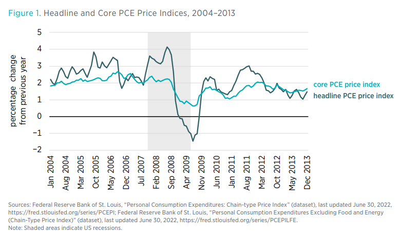
To illustrate how headline and core inflation measures can diverge, figure 1 shows headline and core PCE inflation from 2004 to 2013. For much of the period, headline inflation is greater than core inflation. In early 2008, high energy prices caused headline inflation to be much higher than core inflation, which was relatively steady. As economic contraction greatly worsened later in 2008, headline inflation plunged and even became negative, while core inflation fell more modestly.

With that said, the core measures are still affected by changes in the headline measures to some degree. For example, suppose a war (such as the current war in Ukraine) causes oil production to fall and oil and gas prices to rise. Energy is an input used in the production of other goods, which are included in the core measures. Higher energy prices also make shipping more expensive.

Although the two indices generally follow similar patterns, they differ in several important respects. These differences are categorized in four groups: formula effects, weight effects, scope effects, and other effects.

1. Weight effects. Both the CPI and the PCE are index numbers, which are forms of averages. Each assigns more weight to goods that people buy in larger quantities. For example, people spend more on gasoline than pickles, so gasoline is more heavily weighted than pickles. Each index has a different method of determining the appropriate weights. The CPI is based on surveys of what households are buying, whereas the PCE is based on surveys of what businesses are selling.
2. Formula effects. Each index uses a different index-number formula. When the price of one good in the basket rises, consumers purchase less of that good. Whereas the CPI does not take into account consumers’ substitution between goods, the PCE does.
3. Scope effects. The CPI measures only households’ out-of-pocket expenditures on goods and services, but the PCE also includes households’ expenditures covered by other parties. For example, the CPI does not include medical care services provided by employer-provided medical insurance, Medicare, and Medicaid.
4. Other effects. Other differences between the CPI and PCE are mostly minor and have to do with items such as how to handle seasonal adjustments.

Another popular measure of inflation is the GDP deflator. The CPI and PCE specifically measure consumer prices. Although consumption makes up most of GDP, GDP also consists of investment, government spending, and net exports. Unlike the CPI and PCE, the GDP deflator includes prices of nonconsumer goods such as business equipment. The GDP deflator arguably gives a better sense of inflation than the other indices, but it is less relevant to most people.

Like GDP data, GDP deflator data come out only quarterly, whereas CPI and PCE data come out monthly. This timing is perhaps another reason that the GDP deflator is less commonly cited than the CPI and PCE.

What Causes Inflation?

Milton Friedman, the late Nobel Prize–winning economist, famously coined the saying, “inflation is always and everywhere a monetary phenomenon.” By this, he meant sustained money supply growth is what drives sustained inflation. This claim is true in the long run. In the short run, changes in inflation are more complicated, but even over short periods, monetary policy is very important. Moreover, the central banks of most developed countries today explicitly target inflation when setting monetary policy. When central banks fail to achieve their inflation target over time, their monetary policy is ultimately to blame.

An identity that economists call the equation of exchange helps one understand this idea:

MV = PY

Here M is the money supply; V is the velocity of money or the rate at which money is exchanged; P is the price level, measured by a price index; and Y is real output or income, usually measured as real GDP. Both sides of the equation equal nominal income or total-dollar spending, usually measured as nominal GDP.

By taking the first difference of the natural logarithm of each variable, one can express the equation in terms of growth rates:

m + v = p + y

Here m is the growth of the money supply, v is the growth of velocity, p is the growth of the price level (inflation), and y is the growth of real output.

From this equation, a dynamic equation of exchange, one sees that inflation depends on the growth of the money supply, velocity, and real income. If the money supply grows more rapidly, inflation will rise, all else constant. If people spend their money more rapidly (i.e., velocity rises), inflation will rise, all else constant. If the economy becomes more productive and real income rises, inflation will fall, all else constant.

Under a commodity standard, where money is defined as a unit of a particular commodity, such as gold or silver, money supply growth is determined by changes in the supply of the money-defining commodity. Historically, countries that faithfully adhered to commodity standards experienced inflation or deflation (negative inflation) over short periods, but they experienced very low, near-zero average inflation because money supply growth was constrained.

Today, all countries use government-issued fiat money, which is not defined in terms of any commodity. Under fiat money, money supply growth is determined by the monetary authority (typically, the central bank) of each country. The central bank has a monopoly on the issuance of base money, which includes currency in circulation and reserves held at the central bank. If the central bank wants to increase the money supply, it usually lowers interest rates under its control and buys financial assets to inject newly created money into the economy. It does the opposite to decrease the money supply.

Although the central bank fully controls the monetary base, it does not directly control the entire money supply. Two of the most common money supply measures or aggregates are M1 and M2, which are reported by the Fed. Up until April 2020, when their definitions slightly changed for a technical reason, M1 included currency in circulation and demand deposits (namely, checking accounts), whereas M2 mainly included M1 plus savings accounts and small time deposits (such as certificates of deposit [CDs]).

Before November 2008, the Fed typically pursued an expansionary monetary policy by buying short-term Treasury bills to push interest rates down to its target, the federal funds rate. Banks had to keep a fraction of this money in reserves to satisfy the Fed’s reserve requirements, but they lent out most of the rest to earn profits. This created a money multiplier where an expansion of the monetary base causes the banking sector to increase the total quantity of loans, which increases the money supply.

Beginning in November 2008, the Fed began to pay interest on reserves high enough to entice banks to maintain large quantities of reserves. This greatly reduced the money multiplier. Now when the Fed pursues an expansionary monetary policy, it does so primarily by reducing the interest it pays on reserve balances to encourage banks to increase the size of their loan portfolios and boost the money supply.

Though M1 and M2 are the most well-known measures of the money supply, they are not the only measures. Some central banks publish broader measures called M3 and M4. These measures include other assets such as repurchase agreements (repos), which large financial institutions use to finance loans. Although the Fed no longer reports these broader measures for the United States, the Center for Financial Stability, a nonprofit think tank, reports both the narrower measures the Fed already supplies as well as the broader measures. Notably the Center for Financial Stability’s methodology for measuring the money supply differs from the Fed’s. The Fed’s aggregates are simple-sum measures in that individual components of the money supply are weighted equally. For example, currency, which pays no interest and is highly liquid, is weighted the same as CDs, which pay interest and are less liquid. The Center for Financial Stability publishes Divisia measures, which take varying liquidity into account.

The central bank does not determine how much people choose to put into the accounts that make up any of the monetary aggregates. However, by manipulating the monetary base and by communicating what it expects the course of monetary policy to be, it exerts strong influence on every measure of the money supply.

When the money supply rises, members of the public then have larger money balances, which they can spend on goods and services. As people increase their spending, nominal GDP rises. Although a more expansionary monetary policy can temporarily cause real GDP to rise too, its effect on real GDP, which is ultimately determined by nonmonetary factors, is limited. If nominal GDP keeps growing, people will bid up prices as goods and services become increasingly scarce. This causes inflation to rise. Moreover, if people believe inflation will be high in the future, they will be more likely to spend their money today, making inflation a self-fulfilling prophecy. An important implication here is that a central bank needs to be perceived as credible in stabilizing inflation so it can anchor the public’s inflation expectations.

Because excess nominal GDP growth, which is brought on by excessive money supply growth, is the main cause of inflation, it follows that constraining money supply growth is needed to limit inflation, but economists differ on the best way to achieve this. For much of his career, Friedman argued that the Fed should adopt a constant money supply growth rule where it would increase the money supply by a certain percentage each year. Although this rule may sound appealing, many economists do not recommend this proposal because the relationship between the money supply and inflation is not constant, owing to unpredictable changes in output and velocity.

From the 1990s through the 2010s, many major central banks generally succeeded at producing low inflation. Rather than follow money supply growth rules, they followed—or were at least guided by—Taylor rules, formulas that stipulate what a central bank’s target interest rate should be given certain economic conditions. Taylor rules can be thought of as rules that constrain money supply growth, but they do not imply a particular rate of money supply growth.

Demand-Pull or Cost-Push? The Great Inflation and Today

The preceding analysis is sometimes called a demand-pull explanation because monetary policy is causing aggregate demand to rise and pull up prices. By contrast, some economists argue that inflation is mostly due to cost-push factors. They argue that increases in production costs (e.g., the costs of raw materials and wages) push up prices throughout the economy.

The problem with the cost-push view in explaining persistent changes in inflation is that it relies on microeconomic causes to explain a macroeconomic phenomenon. Cost-push proponents argue that negative supply shocks lead to a wage-price spiral. Suppose an oil shock causes gas prices to rise, and consumers spend a larger share of their budget on gasoline. They then have less money to spend on other goods and services such as groceries, clothes, and restaurant meals. For their demand for these other goods and services not to fall, they will have to demand higher wages from their employer. Employers will then charge higher prices to pay for these higher wages, causing a positive feedback loop between higher prices and wages. However, even if consumers negotiate higher wages, such a loop cannot continue indefinitely purely because of cost-push factors. At some point, employers cannot keep raising wages because doing so will not be profitable, and consumers’ demand for certain goods and services will have to fall. The only way to sustain inflation is to sustain the demand for all goods and services, and the only way to do this is through money creation.

For supply shocks to explain persistent inflation, real GDP would have to persistently fall, which has not happened. Moreover, with some exceptions, changes in real GDP (as well as velocity) tend not to be larger than a few percentage points from year to year.

In the 1970s, some economists, including even Fed Chair Arthur Burns, argued that the high inflation of the time (the Great Inflation) was primarily due to cost-push reasons, including the OPEC (Organization of the Petroleum Exporting Countries) oil shocks and labor unions, rather than demand-pull factors—i.e., expansionary monetary policy. Other economists, notably including Friedman, argued the opposite. One sees clear parallels today as economists debate whether the current inflation is due to disrupted supply chains, the COVID-19 pandemic, the war in Ukraine, monopoly power, or poor monetary policy.

The cost-push narrative of the Great Inflation has some important limitations. Economists point to the mid-1960s as the beginning of the Great Inflation, but the first Middle East oil shock was not until 1973. Furthermore, West Germany, which also experienced the 1973 shock, saw much lower inflation than the United States and other developed countries. This suggests that poor US monetary policy, in contrast to West Germany’s superior policy, better explains inflation than do high oil prices.

The dynamic equation of exchange shows that demand-pull factors were more important than cost-push factors in explaining the Great Inflation. From Q1 1967 to Q2 1982, average inflation as measured by the GDP deflator was 6.39 percent, average real output growth was 2.73 percent, average Divisia M4 (the broadest available measure of money supply) growth was 6.57 percent, and average Divisia M4 velocity growth was 2.55 percent. Although this period saw four recessions, average real output growth was still positive, which would have put downward pressure on the price level. Therefore, strong positive money supply growth and modestly positive velocity growth more adequately explain inflation than do supply shocks.

For the more recent inflationary period, because the Fed pursued a very expansionary monetary policy beginning in March 2020, it makes sense to include data beginning then. From Q1 2020 to Q2 2022, average inflation was 3.13 percent, average real output growth was 1.47 percent, average Divisia M4 growth was 15.27 percent, and average Divisia M4 velocity growth was −10.67 percent. Again, money supply more adequately explains inflation than do supply shocks.

Notably, real growth in 2021 was the strongest annual growth since 1984, owing in large part to the fact that the economy was recovering from the steep COVID-19 pandemic-induced recession in 2020. It is probable that growth would have been even higher had supply chain disruptions not occurred and the effects of the pandemic been smaller. In 2021, the price level overshot its prepandemic trend by the second quarter, but nominal GDP did not overshoot its prepandemic trend until much later in the year. This indicates that negative supply shocks substantively contributed to inflation early in 2021, but it should have been clear by later in the year that inflation was becoming mostly driven by monetary policy.

Central Banks as Inflation Thermostats

Central banks do not directly control any of the variables in the equation of exchange. However, with their monopoly on the issuance of base money, they can determine the size of the money supply, albeit not precisely.

Through their ability to adjust the money supply, central banks can always affect nominal variables or variables denominated in current prices. Thus, they can target any of the following: the price level (P), the growth rate of the price level or inflation (p), nominal GDP (PY), or the growth rate of nominal GDP (p + y).

As mentioned earlier, most central banks target a specific inflation rate when setting monetary policy. This practice started with the Reserve Bank of New Zealand when it formally adopted a 2 percent inflation target in 1989. Most other central banks of major economies have inflation targets at or around 2 percent. Before August 2020, the Fed had a simple inflation target where it would attempt to achieve 2 percent inflation each period without considering previous misses of the target. In August 2020, after years of generally undershooting this 2 percent target, the Fed transitioned to a flexible average inflation target where it would make up for previous undershoots of the target to achieve 2 percent inflation on average over time.

In a 2003 op-ed for the Wall Street Journal, Friedman compared the Fed to a thermostat of a house. Just as a well-functioning thermostat keeps the temperature of a house stable by offsetting changes from the external environment, a good inflation-targeting central bank keeps inflation at target by offsetting changes in the other variables in the equation of exchange. For example, if velocity growth rises and output growth remains stable, the central bank should shrink money supply growth to keep inflation stable.

When a person adjusts a thermostat, the thermostat does not change the house’s temperature, instantly. Similarly, a central bank cannot instantly change the inflation rate, so it can be excused for allowing inflation to deviate from target over short time horizons such as a few months. Over longer time horizons, though, it should be able to keep inflation at, or at least very close, to target.

One important implication of the thermostat comparison is that fiscal stimulus should generally not be very effective if the central bank is successful at targeting inflation. Fiscal stimulus is intended to get the public to spend money on goods and services, raising total spending in the economy, which prompts firms to increase output in response to this new demand. However, if the public spends more and raises total spending, then inflation also rises. An inflation-targeting central bank would offset such stimulus to keep inflation at target.

Finally, supply shocks pose a challenge for central banks’ acting as an inflation thermostat. If a large negative supply shock causes output to fall and inflation to rise temporarily, then to keep inflation at target, the central bank must tighten policy. However, this means tightening at a time the economy is already weakening, and such an action could reduce growth and raise unemployment. Economists generally recognize this concern, which is why they argue central banks should have flexible targets, where they overlook such shocks. However, doing so is difficult in real time. Some economists have pointed to this as a major reason that central banks should switch from inflation targeting to nominal GDP targeting; the latter does not require judgments about changes in inflation from supply shocks.

Political Pressure and Inflation

Political pressure can undermine a central bank’s ability to pursue a sound monetary policy. Although many economists argue central bank independence from politics leads to greater macroeconomic stability, no central bank, the Fed included, is completely insulated from politics.

For example, President Richard Nixon famously pressured Fed Chair Burns to pursue an expansionary monetary policy to boost Nixon’s reelection chances in the 1972 election. Burns proceeded to pursue such a policy, which led to a steep rise in inflation. Although it is not entirely clear whether Burns might have pursued such a policy irrespective of Nixon’s pressure, it is plausible that Burns might have instead pursued a more contractionary policy.

Though more recent presidents have generally accepted the notion of Fed independence (at least in their public statements), President Donald Trump frequently and publicly criticized Chair Jerome Powell for not pursuing a more accommodative monetary policy.

Politicians also face a temptation to pressure central banks to keep deficit financing costs down by buying government bonds, thus lowering the interest rates on those bonds. Fiscal dominance refers to situations where a government forces the central bank to pursue an expansionary monetary policy to sustain fiscal policy. In extreme cases when a government cannot service its debts through taxation or borrowing, it may turn to money creation as the primary means of funding fiscal policy.

Fiscal dominance scenarios frequently lead to very high inflation and even hyperinflation (inflation greater than 50 percent per month). Even if a government is not near a fiscal dominance scenario, it should still practice fiscal restraint to avoid that mere possibility.

Costs of Inflation

The amount of harm from inflation depends on the degree to which the actual inflation rate differs from the expected or anticipated inflation rate. When inflation is at or around its expected rate, its costs are lower. When inflation is very different from its expected rate, its costs are higher.

Expected Inflation

When borrowers and lenders enter multiyear debt contracts, they typically must estimate what inflation will be because contracts are not usually inflation adjusted. For example, when a borrower applies for a 30-year fixed-rate mortgage from a bank, the bank wants to charge a sufficient interest rate to preserve the real (inflation-adjusted) interest rate. If inflation rises but is expected, those who have entered contracts do not suffer because they factored in higher inflation when signing.

There are still costs to higher inflation even when it is expected. First, inflation is effectively a tax on cash, and cash pays no interest. Although such a tax may be less of a problem today than it was in the past (given that society has become increasingly cashless), a nontrivial percentage of transactions are still done in cash. According to a recent Fed study, US consumers used cash for 26 percent of all payments in 2019.

Second, when tax rates are not indexed for inflation, higher inflation effectively increases people’s tax burden. Suppose a person’s nominal income rises in response to rising inflation, but her real income remains the same. If taxes were not indexed for inflation and her higher nominal income were to push her into a higher income tax bracket, she would be taxed at a higher rate, despite not earning more in real terms. The Economic Recovery Tax Act of 1981 partially addressed this problem by indexing federal income tax brackets. However, the tax on investment income, including interest, dividends, and capital gains, is not indexed for inflation. This discourages savings.

Third, firms must change their listed prices more frequently in response to inflation. These costs are called menu costs (getting their name from restaurant menus), but they include the changes to all prices throughout the economy (e.g., prices on the price tags at brick-and-mortar stores, prices online, prices on gas station signs).

Unexpected Inflation

When inflation is not expected, the same problems as in the expected case still apply, but now there are greater costs. At least one party in any debt contract is worse off. If inflation is higher than expected, a borrower owes less in real terms, and the lender is worse off. If it is lower than expected, the borrower is worse off because he or she owes more in real terms, whereas the lender is better off.

Uncertainty about future inflation means that parties will be less likely to enter debt contracts because lenders will be less confident that such contracts will be profitable. The longer the maturity of a contract—whether for a corporate bond or a personal loan such as a mortgage—the greater the risk of that contract. Inflation adds to this riskiness.

Higher, more volatile inflation also adds to so-called noise in prices. It is not clear whether prices for particular goods are rising because they reflect changes in supply and demand for those goods or because of inflation. Thus, it becomes more difficult to make investment decisions.

By interfering with the price system and financial markets, high inflation makes longer-term economic planning very difficult and discourages savings and investment, which are critical for long-run economic growth.

Benefits of Inflation?

There is universal agreement that high inflation is very harmful and should be avoided, but economists debate whether low inflation can have any benefits.

In the 1960s, many economists believed in an early version of the Phillips curve, which depicts a permanent tradeoff between unemployment and inflation: if unemployment is too high, it can be lowered in exchange for higher inflation, and vice versa. This belief was proven false in the 1970s when both inflation and unemployment rose.

Economists revised the model and now argue that although inflation above its expected rate can temporarily reduce unemployment, unemployment cannot remain below a natural rate determined by nonmonetary factors such as workers’ level of education. Similarly, inflation below the expected rate can temporarily raise unemployment. For this reason, many economists argue that below-target inflation is undesirable unless it is caused by a benign supply shock (i.e., an improvement in productivity).

This argument for avoiding surprisingly low inflation is reasonable, but it raises a question: why target and anchor inflation expectations around a positive rate in the first place?

There are two main arguments for slightly positive inflation. The first is that slightly positive inflation lubricates labor markets. This is essentially a psychological argument. If employers wish to cut real wages in response to other changing prices, they can do so without cutting nominal wages, which could undermine workers’ morale and reduce productivity.

The second argument is that slightly positive inflation can help central banks better implement monetary policy. As evidence for this claim, some economists point to the Fisher effect: