The Stance of Monetary Policy: The NGDP Gap

*Updated May 11, 2020

One of the most important questions facing the Federal Reserve (Fed) is also one of the hardest for it to answer: What is the current stance of monetary policy? The answer to this question is straightforward in theory, but is quite challenging to apply in practice. Despite many valiant efforts by central bankers, academics, and market participants, there is still a lot of uncertainty in real time about whether monetary policy is too tight, too loose, or just about right. This policy brief attempts to add some clarity to this question by providing a new measure of the stance of monetary policy.

This policy brief specifically shows how to construct a benchmark growth path for nominal GDP (NGDP) where monetary policy is neither expansionary nor contractionary. Deviations of actual NGDP from this neutral level of NGDPprovide a way to assess the stance of monetary policy. These deviations, called the NGDP gap, can be used by the Federal Open Market Committee (FOMC) as a cross-check on existing indicators of the stance of monetary policy.

This new measure does not require knowledge of standard macroeconomic policy indicators such as r-star (the neutral real interest rate) or y-star (potential real GDP), and therefore avoids the challenges of “navigating by the stars” as outlined by Fed chair Jerome Powell. All it requires are some simple calculations applied to publicly available forecasts of NGDP. Despite its simplicity, the NGDP gap can be motivated from both New Keynesian and monetarist theory, and therefore can serve as a useful metric in these frameworks.

Since NGDP comprises both real GDP and the price level, it captures both elements of the Fed’s dual mandate. NDGP is also a dollar-based or a nominal variable, and therefore can be shaped by the Fed over the long run. The FOMC, consequently, can use the NGDP gap as a practical guide to the stance of monetary policy in a manner consistent with its congressional mandate. The FOMC’s use of the NGDP gap, moreover, does not require the adoption of a NGDP target by the Fed.

To promote the use of this new measure, the Monetary Policy Program at the Mercatus Center at George Mason University will provide regularly updated data for the neutral level of NGDP and the NGDP gap on its website. The website will provide both real-time vintage data and the latest quarterly data. The calculations behind the new measures will also be made available so that the data will have complete transparency.

This policy brief shows the rationale and construction of this benchmark path for NGDP and how it can be used to gauge the stance of monetary policy. It then discusses how the NGDP gap implied by this measure fits into the New Keynesian and monetarist frameworks, as well as a financial stability framework. Finally, this policy brief shows how the NGDP gap could help policymakers during the COVID-19 crisis.

The Neutral Level of NGDP: Rationale and Construction

The NGDP gap, as noted above, is the deviation of actual NGDP from its neutral level. The neutral level of NGDP, in turn, is the public’s expected growth path of nominal income. The rationale for this definition is twofold. First, members of the public make many economic decisions on the basis of forecasts of their nominal incomes. For example, households may take out mortgages and car loans on the basis of forecasts of their nominal income. Similarly, firms may finance with debt and commit to multiyear contracts on plants, raw materials, and labor on the basis of forecasts of their nominal income. Second, the actual realization of nominal incomes may turn out to be very different from what is expected and, as a result, may be disruptive for households and firms that are not be able to quickly adjust their economic plans. These disruptions can be avoided by maintaining NGDP on the growth path expected by the public.

To be clear, each household and firm will have an idiosyncratic component to its nominal income forecast, but there will also be a common component reflecting broader nominal income trends. Research has shown, for example, that across all age, income, and education groups of consumers, expected nominal incomes fell at a similar pace during the Great Recession and contributed to the decline in aggregate consumption. It is this common component that the Fed can shape and that is reflected in aggregate nominal income forecasts.

In calculating the neutral level of NGDP, it is important to remember that in addition to the nominal income forecasts made in the current period, there will be nominal income forecasts made in subsequent periods that are for the same future date. Future periods, in other words, may have many different nominal income forecasts applied to them with each forecast, leading to potentially new and different economic decisions. Given this possibility, it makes sense to take an average of the different nominal income forecasts being applied to the same period.

To capture these ideas, an average forecast of nominal income for each period is created that is based off forecasts for that period from the preceding 20 quarters. This five-year forecast horizon is chosen because it assumes that all constraints created by decisions based on a forecast can be fully unwound within five years. Each period’s average forecast uses median forecast data from the Federal Reserve Bank of Philadelphia’s quarterly “Survey of Professional Forecasters”(SPF) and is constructed in three steps.

First, for each period, 20 quarters of NGDP growth forecasts are created using short-run NGDP forecasts as well as long-run NGDP forecasts found in the SPF. The short-run NGDP growth forecasts are explicitly provided by the SPF for the first five quarters (t + 1 to t + 5). The long-run NGDP growth forecasts are not explicitly provided in the SPF, but are implied by the combination of the 10-year GDP deflator inflation and 10-year real GDP growth forecasts in the SPF. This implied long-run NGDP growth forecast provides an annual average forecast that is used for all the remaining 15 quarters (t + 6 to t + 20). Together, these series provide 20 quarters of forecasted NGDP growth, as shown in table 1.

Second, the NGDP growth rate forecasts are turned into dollar-level NGDP forecasts by taking the current dollar value of NGDP at time t and sequentially expanding it by the forecasted growth rates for periods t + 1 to t + 20. This process creates a 20-quarter forecast path of NGDP in dollar form. These 20 forecasts are created for every period, starting in the first quarter of 1992, when the data become available.

Third, an average dollar forecast for a given quarter is created using all the dollar forecasts for that period from the previous 20 quarters. For example, the average NGDP forecast for the first quarter of 1997 is the average of every forecast created for that period starting in quarter 1, 1992, and going through quarter 4, 1996. This step is repeated for every period, so that a new average forecast series is created. This new time series is the neutral level of NGDP. It can be summarized as follows:

Figure 1 shows the resulting neutral level series as well as the NGDP gap, the percent difference between the actual level of NGDP and the neutral level. The NGDP gap measures the difference between what the public, on average, thought nominal income would be in a particular period and what it actually turned out to be. It can be viewed, consequently, as a nominal income shock or, equivalently, as an aggregate demand shock. To the extent that monetary policy is driving NGDP, it can also be seen as the stance of monetary policy.

Several features stand out in figure 1. First, the neutral level (panel A) shows that eventually the lingering effects of past forecasts fade and converge with actual NGDP, a kind of long-run money neutrality feature. Second, the NGDP gap series (panel B) shows a boom and bust cycle that corresponds with the US business cycle. Specifically, the figure shows positive gaps during the booms in the late 1990s and in the first few years of the 21st century as well as a large negative gap during the Great Recession. The NGDP gap series also shows a slow recovery after 2009, and shows the “mini-recession” of 2016. The NGDP gap starts flatlining in 2018 after the Fed interest rate hikes, leaving it just below the neutral mark of 0 percent.

The NGDP gap, therefore, captures many of the features of the business cycle and provides another useful crosscheck on the stance of monetary policy. Unlike other measures that require estimates of r-star or y-star, this measure is simple to calculate and uses publicly available data. This measure, moreover, can be motivated from standard monetary frameworks, as shown in the sections that follow.

The NGDP Gap: A New Keynesian Interpretation

The New Keynesian approach to macroeconomics is the dominant view inside most central banks. This framework requires the use of unobservable variables that have to be estimated, including the output gap and the neutral real interest rate. The output gap is especially important and appears in every equation of the New Keynesian three-equation workhorse model: it helps determine inflation in the New Keynesian Phillips curve, it helps shape monetary policy in the Taylor rule, and it is tied directly to the expected path of monetary policy in a forward-solved expectational IS curve.

The output gap, then, is an integral part of the New Keynesian framework. It is defined as the percent difference between actual and potential real GDP and reveals whether the economy is running hot (a positive output gap) or cold (a negative output gap). Whether an economy is running hot or cold, in turn, depends on whether there is a shortfall or excess of aggregate demand in the economy. As noted earlier, the NGDP gap is a nominal income shock that is equivalent to an aggregate demand shock. Consequently, the NGDP gap fits well into the New Keynesian framework as an indirect measure of the output gap.

In fact, as shown in figure 2, the NGDP gap (panel A) and an average of the output gaps from the Congressional Budget Office, the International Monetary Fund, and the Organisation for Economic Co-operation and Development are very similar, with a contemporaneous R² of 73 percent. The relationship is even stronger with a two-quarter lag of the output gap being related to the current NGDP gap, with an R² of 88 percent. The NGDP gap, therefore, can be viewed as a simple alternative way to measure the output gap in the New Keynesian model.

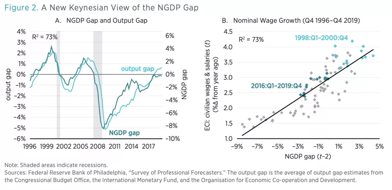
Interestingly, the NGDP gap also has a strong relationship with nominal wage growth, as measured by the employment cost index for civilian salaries and wages (ECI). The NGDP gap (panel B) has an R² of 73 percent with a two-quarter lag of the year-on-year growth rate of the ECI. The chart shows that the difference between the modest wage growth over the past few years (dark-teal diamonds) and the higher wage growth of the late 1990s (light-teal diamonds) can be readily explained by the NGDP gap. This finding is consistent with the research of Adam Ozimek and Ernie Tedeschi, who argue that it is easier to understand lackluster wage growth over the past decade once a proper measure of slack or, alternatively, aggregate demand shortfall is used in Phillips curve–type analyses.

The NGDP Gap: A Monetarist Interpretation

Monetarists as far back as Milton Friedman see the stance of monetary policy as the gap between the money supply and real money demand. If the money supply is expected to be below real money demand, then monetary policy is tight, and vice versa. If the money supply and real money demand converge, then monetary policy is neutral.

Monetarists, however, are no different than New Keynesians in that their framework depends on a latent variable: real money demand. Like the output gap, real money demand is determined by the fundamentals of the economy, can quickly change, and is not directly observable. A simple workaround is to observe that the equation of exchange identifies NGDP as the money supply automatically adjusted for velocity (i.e., M_tV_t = P_tY_t = NGDP_t) Velocity, V_t, measures how many times the money stock is used in a given period, and therefore is an indicator of real money demand. From a monetarist’s perspective, then, NGDP provides a robust way to assess the stance of monetary policy, since it is effectively the velocity-adjusted money supply.

This understanding can be expanded in light of the neutral level of NGDP. As noted above, the neutral level of NGDP is where NGDP should be, given the public’s past forecasts of NGDP. If NGDP is not at its neutral level, then its components—the money supply and velocity—must not be at their neutral levels. If the neutral level of velocity is defined as velocity’s trend value, then the neutral money supply falls directly out of the equation of exchange, given the knowledge of neutral NGDP.

 Now take the percent difference gap between these measures and their actual values and sum them up to get the NGDP gap:

The NGDP gap, then, can be derived from the traditional monetarist’s perspective. Moreover, Joshua Hendrickson shows that the NGDP gap can also be motivated from the newer monetary search models used in the New Monetarism literature. The NGDP gap, then, could be viewed as the monetarist’s version of a simple metric that reflects the stance of monetary policy, similar in spirit to what the Phillips curve or the forward-solved expectational IS curve does for the New Keynesian framework. Put differently, if central bankers wanted a quick monetarist’s take on monetary policy, they could look to the NGDP gap for the answer.

Figure 3 takes the decomposition of the NGDP gap found in equation (3) and applies it using the Divisia M4 money supply. This is a very broad measure of the money supply that includes retail and institutional money assets and is constructed according to the Divisia index method. Specifically, figure 3 shows the relative contributions of the velocity and money supply gaps to the NGDP gap. Panel A shows that the velocity gap plays an important role in the business cycle, contributing to the wide swings in the NGDP gap. During the Great Recession, for example, it was the main cause of the initial sharp decline in aggregate demand. Put differently, there was a large real money demand shock between 2006 and 2008, a result consistent with the run on the financial system during the early stage of the recession. Panel B indicates that the slow recovery from the Great Recession, on the other hand, was due to a drop in the money supply, which only slowly recovered.

Ostensibly, the two developments are related—the run on the financial system caused by the real money demand shock destroyed some of the institutional money assets and thus lowered the Divisia M4 money supply—but this decomposition provides a convenient way to think about the stance of monetary policy from a monetarist’s perspective.

The NGDP Gap: A Financial Stability Interpretation

The monetarist discussion earlier alludes to a potential link between the NGDP gap and financial stability. Research from several quarters confirms this link. Hitting the public’s expected growth path of nominal income is important to achieving financial stability. The basic idea is that in a world of incomplete financial markets, where one cannot insure against all future risks, maintaining nominal income on its expected growth path will lead to better risk sharing between debtors and creditors. This outcome happens since a stable nominal income level will lead to countercyclical inflation and, as a result, to procyclical real debt burdens. As a result, debtors will benefit during recessions and creditors will benefit during booms.

As an example, assume there is a negative supply shock that unexpectedly lowers real GDP. If the Fed keeps nominal income on its expected growth path so that it does not fall, then inflation will temporarily rise. The unexpectedly higher price level will allow the debtor to make a lower real debt payment to the creditor. The real income loss is therefore more evenly shared between the debtor and the creditor. Conversely, assume there is a positive supply shock that unexpectedly raises real GDP. If the Fed keeps nominal income from rising above its expected growth path, then inflation will temporarily fall. The unexpectedly lower price level will cause the debtor to make a higher real debt payment to the creditor. This way, the creditor gets to share in some of the unexpected “windfall gains” in the economy, despite having funds locked up in a lower-yielding fixed-price nominal debt contract.

What these scenarios show is that a highly leveraged world can be turned into an equity-like world by maintaining the expected growth path of nominal income. This transformation should promote financial stability. Along these lines, in a 2019 study I provided cross-country evidence that the closer a country’s NGDP was to its precrisis expected growth path, the better its financial system fared during the Great Recession. In other words, the closer a country’s NGDP gap was to 0 percent, the more resilient was its financial system.

The NGDP gap, therefore, should be correlated with financial activity and can be used in assessing the health of the financial system. Figure 4 provides some evidence consistent with this interpretation. Panel A shows the year-on-year growth of credit to the nonfinancial private sector in the United States. There is a strong relationship, with an R² of 81 percent. Panel B shows the rate of nonperforming loans in the United States. It too comes in with a strong relationship, with an R² of 83 percent. While one has to be careful about drawing conclusions about causality on the basis of these charts, it is important to remember that the NGDP gap is partly the product of a forecast going back five years. This suggests there is some causality flowing from the NGDP gap to the financial indicators, a point borne out in the more careful causal analysis of my 2019 study. The NGDP gap, then, can be a helpful part of financial stability analysis.

Robustness Check

One concern about the NGDP gap is how useful it is in real time. All the figures so far show the NGDP gap using the most current data. It is well known that GDP data, including NGDP, are released by the Bureau of Economic Analysis in three stages: the advance, preliminary, and final estimates. The estimates are sequentially released months after the quarter ends. Typically, each estimate is a revision of the previous one. The bureau further revises its estimate of NGDP in the years that follow. So it is not clear how useful the NGDP gap would be in real time before the revisions are made.

Figure 5 addresses this concern by showing the current NGDP gap against two real-time measures using vintage NGDP data. The first one, Vintage NGDP Gap 1, takes the initial-release NGDP data for each quarter to construct an NGDP gap. In other words, it shows the NGDP gap policymakers would have seen in real time given the initial NGDP data. This series, however, has a limitation. For a given quarter, the initial release comes months after the quarter ends. If you are a policymaker in the midst of an important turning point in the economy, this delay may be costly.

Consequently, a second real time series called Vintage NGDP Gap 2 is provided. This series takes the Vintage NGDP Gap 1 from the previous quarter and uses it to predict the current quarter using a simple autoregressive model. For example, say it is the third quarter of 2008 and a Fed official is nervously wondering what is happening to the NGDP gap. The Fed official could take the Vintage NGDP Gap 1 from the previous quarter, which is available, and use it to forecast the NGDP gap for quarter 3. The Vintage NGDP Gap 2 replicates this exercise using autoregression with one lag.

Figure 5 shows the results for the whole sample period in panel A and for the Great Recession period in panel B. Panel A shows that the vintage data tracks the current data with a small lag. To see how consequential this lag is, panel B zooms in on what Fed officials would have seen in real time during the pivotal year of 2008. Vintage NGDP gap 1 shows negative values for the NGDP gap through all of 2008; vintage NGDP gap 2 shows negative values beginning in the second quarter of 2008. Though both vintage series fail to fall as fast as the final revised NGDP gap, they both were still showing a contraction in aggregate demand throughout 2008. Between April and October 2008, the FOMC left its interest rate target unchanged at 2 percent because of inflation concerns. Had the committee seen this measure, the data may have encouraged it to rethink the pause in rate cuts. The NGDP gap, then, can be a useful guide to monetary policy in real time.

COVID-19 Crisis

The NGDP gap also has a bearing on the war against the novel coronavirus disease COVID-19. There are two fronts to this war: a public health battle against the virus and an economic battle to save an economy put on lockdown. This lockdown amounts to an economically induced coma, and the financial support coming from Congress and the Fed is a form of life support until the coma is lifted.

This economic life support includes direct cash transfers and unemployment insurance sent to households, grants and loans given to businesses, backstops and investments directed to credit markets, and more. These programs, though far from perfect, are motivated by a desire to maintain household and business nominal incomes so that they can meet their preexisting financial obligations, such as mortgage payments and payroll. Otherwise, there could be widespread bankruptcies and liquidations that permanently harm the economy.

The NGDP gap provides a way to assess whether the financial support from Congress and the Fed is doing its job. If a negative NGDP gap starts to emerge, then nominal incomes will be less than expected, and a debilitating wave of insolvencies and sell-offs will occur. On the other hand, if a persistent positive NGDP gap emerges, then there could be a sustained wave of inflation. The NGDP gap, in short, provides a big-picture way to see how all the various government support programs for the COVID-19 crisis are collectively affecting nominal incomes relative to public expectations.

Conclusion

This policy brief has shown how to construct a benchmark growth path for NGDP that can be viewed as the neutral levelof NGDP. Any deviations of actual NGDP from this neutral level path can be used to assess the stance of monetary policy and, to some extent, to assess financial conditions. This measure is called the NGDP gap and can be used by the FOMC as an important cross-check on existing indicators of the stance of monetary policy. The FOMC’s use of the NGDP gap does not require the adoption of an NGDP target by the Fed.

A great feature of the NGDP gap is that its construction does not require knowledge of unobservable indicators such as the output gap or real money demand. All it requires are simple calculations applied to publicly available forecasts of NGDP. Despite the NGDP gap’s simplicity, it can be motivated from both New Keynesian and monetarist theory, and therefore can serve as a useful metric in these frameworks. It can also be a useful guide to policymakers in their economic fight against COVID-19. 

This new measure will be available online and regularly updated by the monetary policy research program at the Mercatus Center. The website will provide both real-time vintage data and the latest current quarterly data. The calculations behind the new measures will also be made available.

*Note on the Update from May 11, 2020

This policy brief has been updated since its original release. In an earlier version, I used the 10-year CPI inflation forecast. In this update, I use the 10-year GDP deflator inflation forecast to construct the 10-year NGDP growth forecast. Thanks to Evan Koenig for suggesting this improved approach.